A new ice2ice related paper studying the impacts of Arctic sea ice loss is being published in Journal of Climate (currently available as Early Online Release). The paper is authored by ice2ice researchers Rasmus A. Pedersen (NBI/DMI), Peter Langen (DMI) and Bo Vinther (NBI) in collaboration with Ivana Cvijanovic (LLNL, USA).
The analysis is based on general circulation model simulations with CESM in an idealized setup, and investigates the atmospheric response to sea ice loss in different parts of the Arctic.
Three investigated sea ice scenarios with ice loss in different regions all exhibit substantial near-surface warming which peaks over the area of ice loss. The maximum warming is found during winter, delayed compared to the maximum sea ice reduction. The wintertime response of the mid-latitude atmospheric circulation shows a non-uniform sensitivity to the location of sea ice reduction. While all three scenarios exhibit decreased zonal winds related to high-latitude geopotential height increases, the magnitudes and locations of the anomalies vary between the simulations.
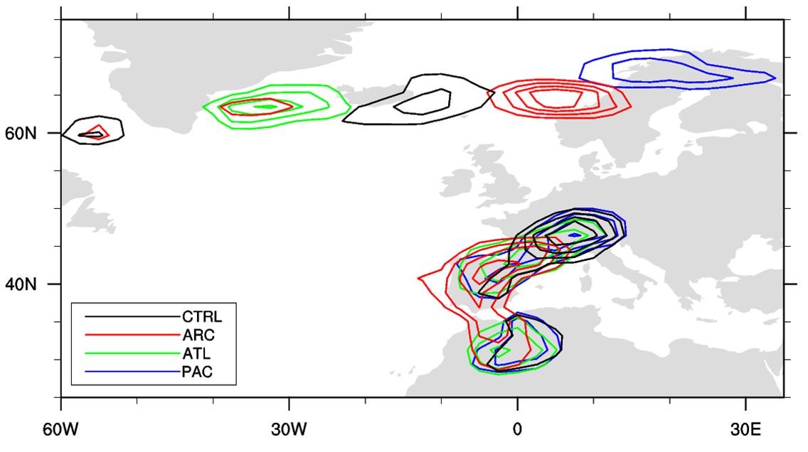
The location of the wintertime (DJF) NAO centers of action are illustrated through the location of the ten highest and ten lowest values of the leading EOF from 500 bootstrap samples. Contours show the total number occurrences in each grid cell combining all bootstrap samples: CTRL (pre-industrial ice cover) in black, ARC (ice loss across entire Arctic) in red, ATL (ice loss in the Atlantic sector of the Arctic) in green and PAC (ice loss in the Pacific sector of the Arctic) in blue. The contour interval is 50 counts with the lowest contour at 50.
Investigation of the North Atlantic Oscillation reveals a high sensitivity to the location of the ice loss. The northern center of action exhibits clear shifts in response to the different sea ice reductions. Sea ice loss in the Atlantic and Pacific sectors of the Arctic cause westward and eastward shifts, respectively.
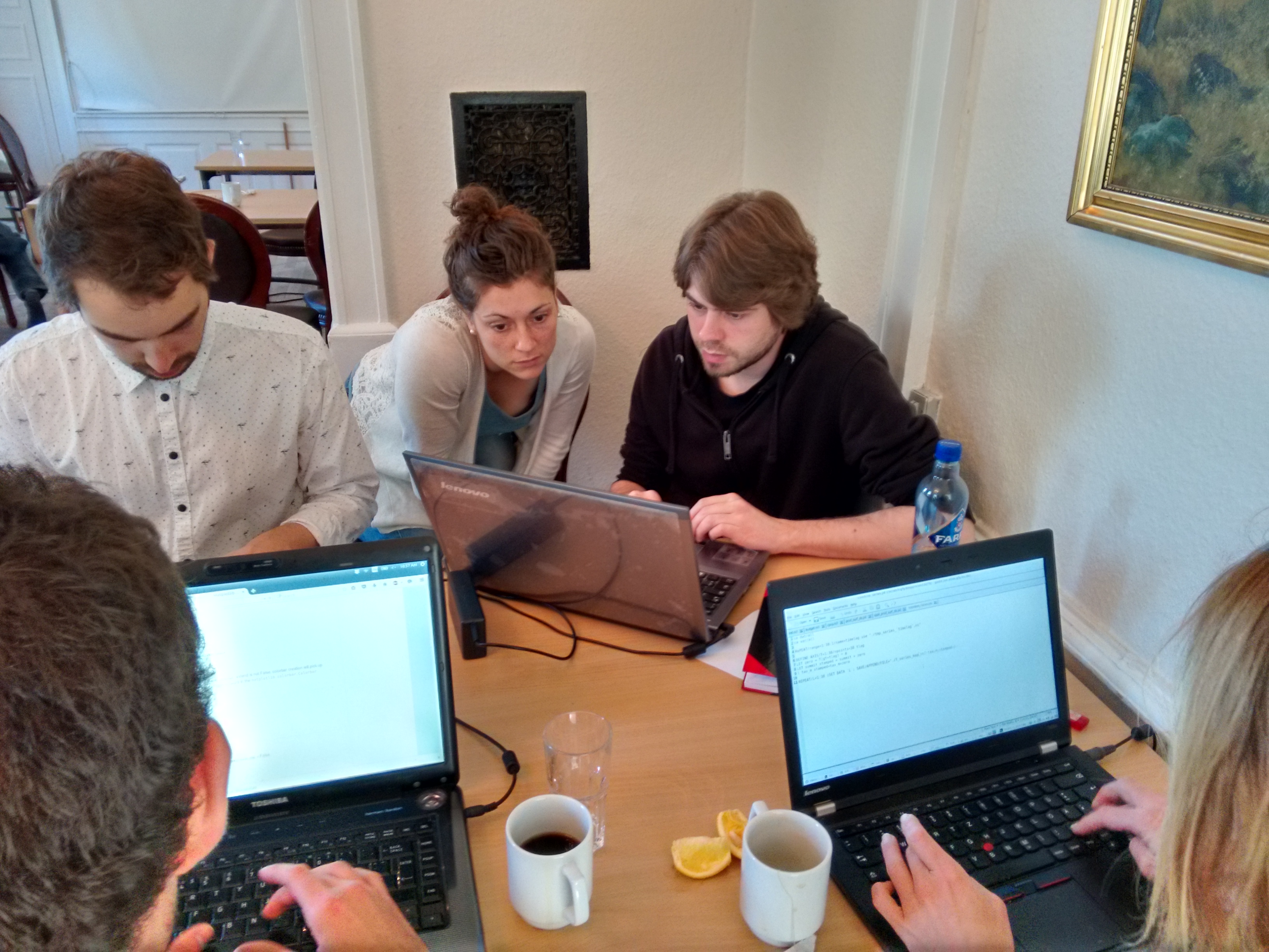
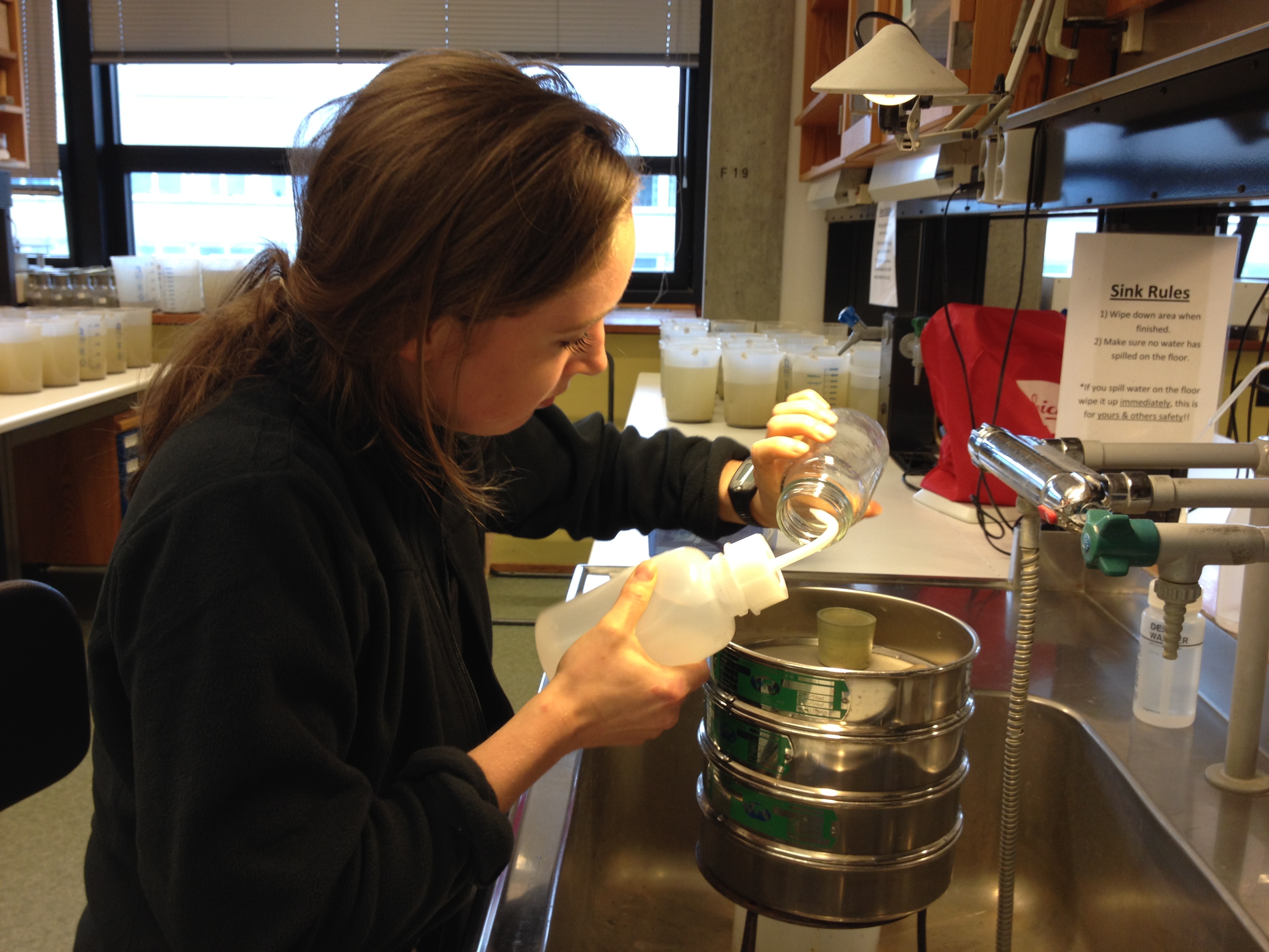
The CFA melting campaign of the Renland ice core started mid-October at the Centre for Ice and Climate (CIC) in Copenhagen. Paul H. and Andreas from Bergen visited the lab early in the campaign and saw first-hand how an ice core is prepared and analyzed. Below is their explanation of the continuous flow analysis ice core lab.
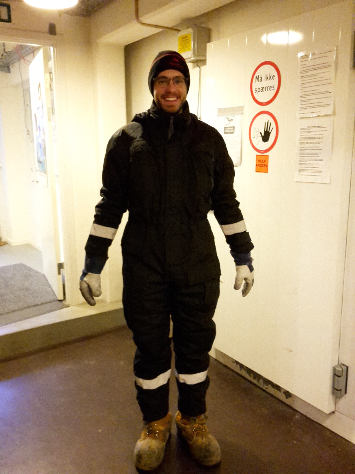
The people at the CFA work in two shifts from 8-14 and from 14-until closing time. During a normal day approximately 16m of ice is being melted. The first part of the work begins in the “warm” freezer at -15°C. The cores are stored in an even colder freezer. So for this work you better pack yourself better than Paul did on his first day.
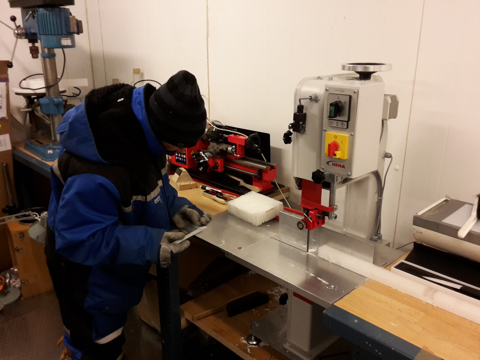
The ice cores are stored in 55cm long pieces; ideally if there are no breaks in between. To get a square-shaped core that fits into the melting frame, part of the core is cut again. Paul V. is showing the newcomer how it is done.
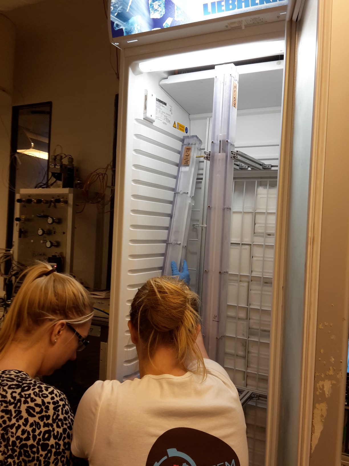
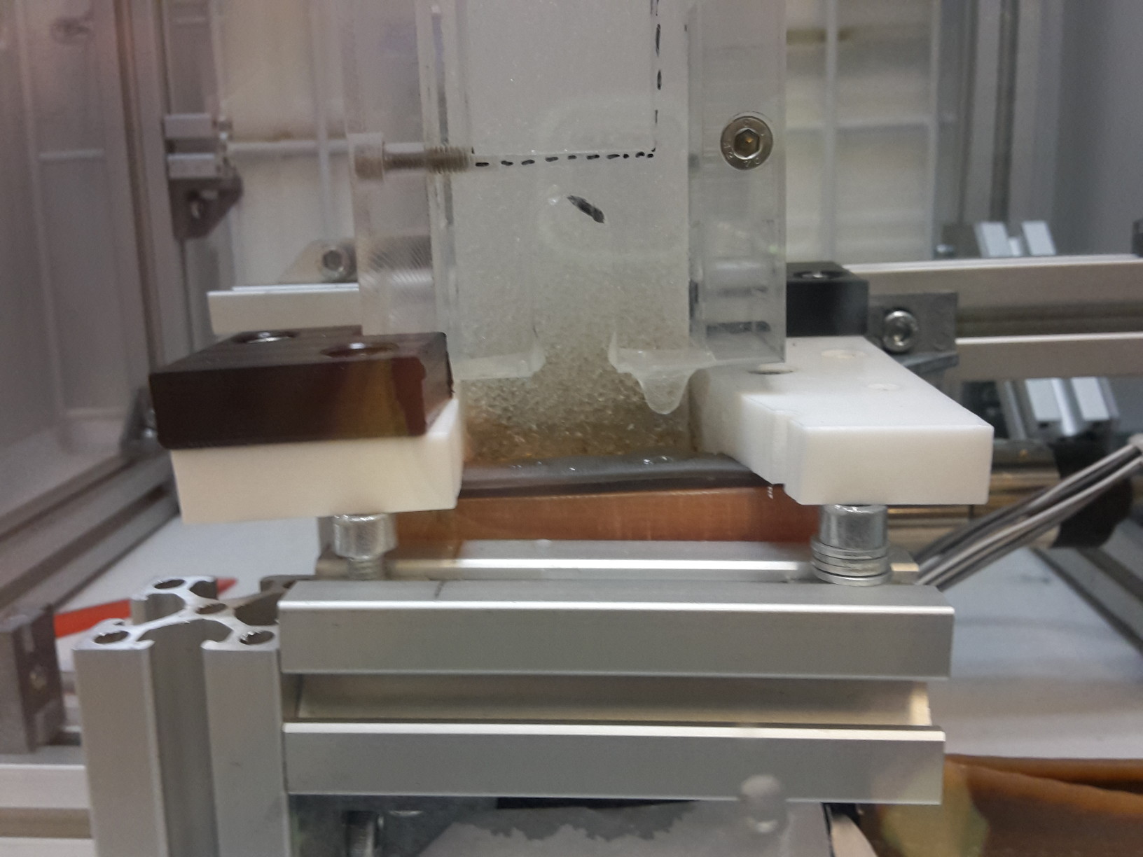
After that the filled melting frames are put in a freezer in the lab where they are melted via the so-called melt head.
The melt rate is governed by the temperature of the melt head. You can nicely see the air bubbles within the ice.
Then the melted ice is separated into a lots of little streams, both gaseous and liquid. The “gas people” measure stable water isotopes (delta_18O, delta_17O, delta_D) as temperature proxies and methane employing laser mass-spectrometry. The “liquid people” measure the sum of all dust, calcium, iron, conductivity, pH, NH4+, sodium, and black carbon, either using direct absorption or fluorescence. All these measurements are done from the continuous sample stream.
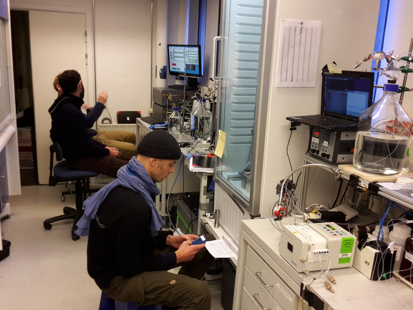
So let’s take a quick look at the lab. Paul watching the ice core has plenty of time to check emails.
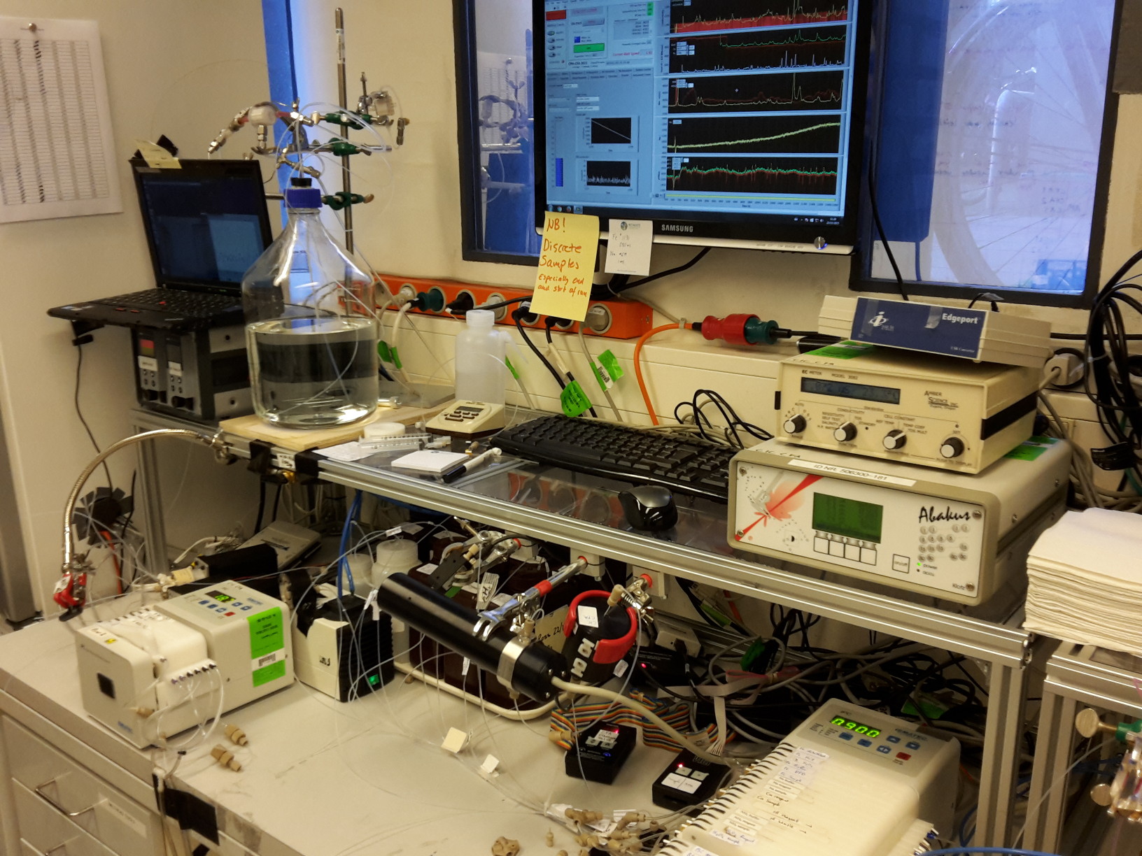
The main screen of the liquid part measurements.
Finally the first part of the black carbon detector is Ross-approved.
Besides all the science, Copenhagen also offers nice sunsets, fantastic cycling, and a great bakery across from the apartment. We limited ourselves to one kanelsnulle per day.
We started to get an appreciation for the astounding amount of work and attention that goes into producing each time series from an ice core. Many thanks to our hosts in Copenhagen for spending the time teaching and talking with us.
Last week several nations met at the danish science society to discuss in more details the plan for the EastGRIP ice core drilling project. The project focuses on the North East Greenland Ice Stream. Several ice2ice members are also part of the EastGRIP project including lead PIs of ice2ice Eystein Jansen (N), Bo Vinther (DK) and Kerim Hestnes (DK)
Several danish news blogs picked up on the information amongst them the danish national television that had a 6 minutes long interview with lead scientist of the EGRIP project Dorte Dahl-Jensen (link-aprox 25 minutes in).
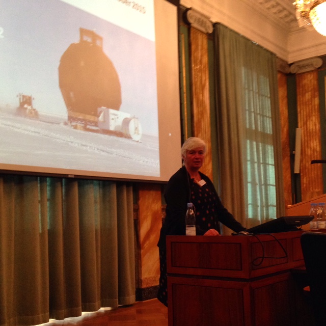
Twenty scientists gathered in Copenhagen at the end of October 2015 to discuss the most recent isotope model developments and the most recent scientific understanding and interpretation of the d18O changes recorded in Greenland during the last deglaciation.
The cryosphere is in fast transition and there is the possibility that the ongoing rapid demise of Arctic sea ice may instigate abrupt changes on the Greenland Ice Sheet. Ice cores here show clear evidence of past abrupt warm events with up to 15°C warming in less than a decade, most likely triggered by rapid changes in Arctic sea ice.
These results rely heavily on oxygen isotope data, which is a key climate proxy from ice cores as well as marine sediment cores. Over the last two decades there have been a number of studies with climate models investigating the possible mechanisms behind these large changes in climate. However, comparing reconstructed climate as recorded by the oxygen isotope record with the physical climate as given by the numerical models is a challenge.
The group focused on future research priorities to answer some key questions:
How can models help us better understand the rapid changes in d18O?
How changes in local and non-local processes play a role in affecting the d18O recorded over Greenland during rapid abrupt cooling events?
What are the biggest uncertainties and challenges in the isotope modelling community?
Additional key questions were:
What was the role of sea-ice cover in affecting the d18O recorded during the D-O events?
How the changes in sea-ice extent affect the origin of moisture delivered over Greenland?
Sensitivity studies exploring the above-mentioned aspects might be model dependent. Hence, it is important to investigate them in a multimodel framework. For this reason, a set of sensitivity studies with common boundary conditions has been defined and they will be run by 4 different modelling groups (CESM, GISS, ECHAM, HadGEM (?)). The results of these simulations will then be discussed in a future workshop within the Ice2ice project.
Author: Francesco S. R. Pausata, Department of Meteorology and Bolin Centre for Climate Research, Stockholm University, Stockholm, Sweden; email: francesco.pausata@misu.su.se
A bootcamp for the ice2ice PhDs took place in Nothern Sealland, Denmark. 17 phd’s and 5 mentors participated in the workshop that lasted 5 days. Below a report from the Phd’s.
Day 1. Monday, September 28th
From Copenhagen, we drove 1.5 hrs to Anneberg hostel on Nord-Sjælland, where we would spend the whole week. Following a group lunch, we made a quick introduction round and started right away with short presentations of the three workshop groups:
Ocean temperature during Dansgaard–Oeschger (DO) events – DO dynamics debated; simulation of full DO cycle challenging – proxy surrogate method – model data pool vs. proxy data pool (resolution 1-2 degrees) – model run that fits proxy data – spatial consistency?
Sea Ice and Greenland accumulation – How is sea ice influencing accumulation on Greenland? Spatial correlation between sea ice and accumulation; investigate influence of delay; investigate possible mechanisms for accumulation-sea ice connection
Inverse modeling of ice shelves – explicit focus on method (inversion – i.e. invert surface velocity fields for viscosity or basal friction to best fit observed velocities) – inverse theory + real world experiments in Antarctica (no present-day ice shelves in Greenland)
Photo credit:Henning Åkeson
The introduction of the workshop groups was followed by our first science talk by Camille Li. Camille gave a quick introduction to the climate system and how to come from the real world to a climate model.
Day 2. Tuesday, September 29th
The morning started with a science talk by Chris Borstad, who talked about changes in ice shelf rheology.
Afterwards, the group work started with a meeting with the mentors, and the session lasted until dinner. The evening consisted of a data visualization workshop. Here Aleksi showed different approaches to plot flow patterns when making geographic maps. Camille Li showed plots from her contribution to the IPCC (2014) report about temperature and precipitation response to freshwater hosing (8.2 ka event). Henning talked about color graphics in plotting, and introduced a MATLAB function that always created the most distinguishable colors when plotting. Chris talked about how the choice of colormap should depend on the data, and why the color scale can perceive the reader.
Day 3. Wednesday, September 30th
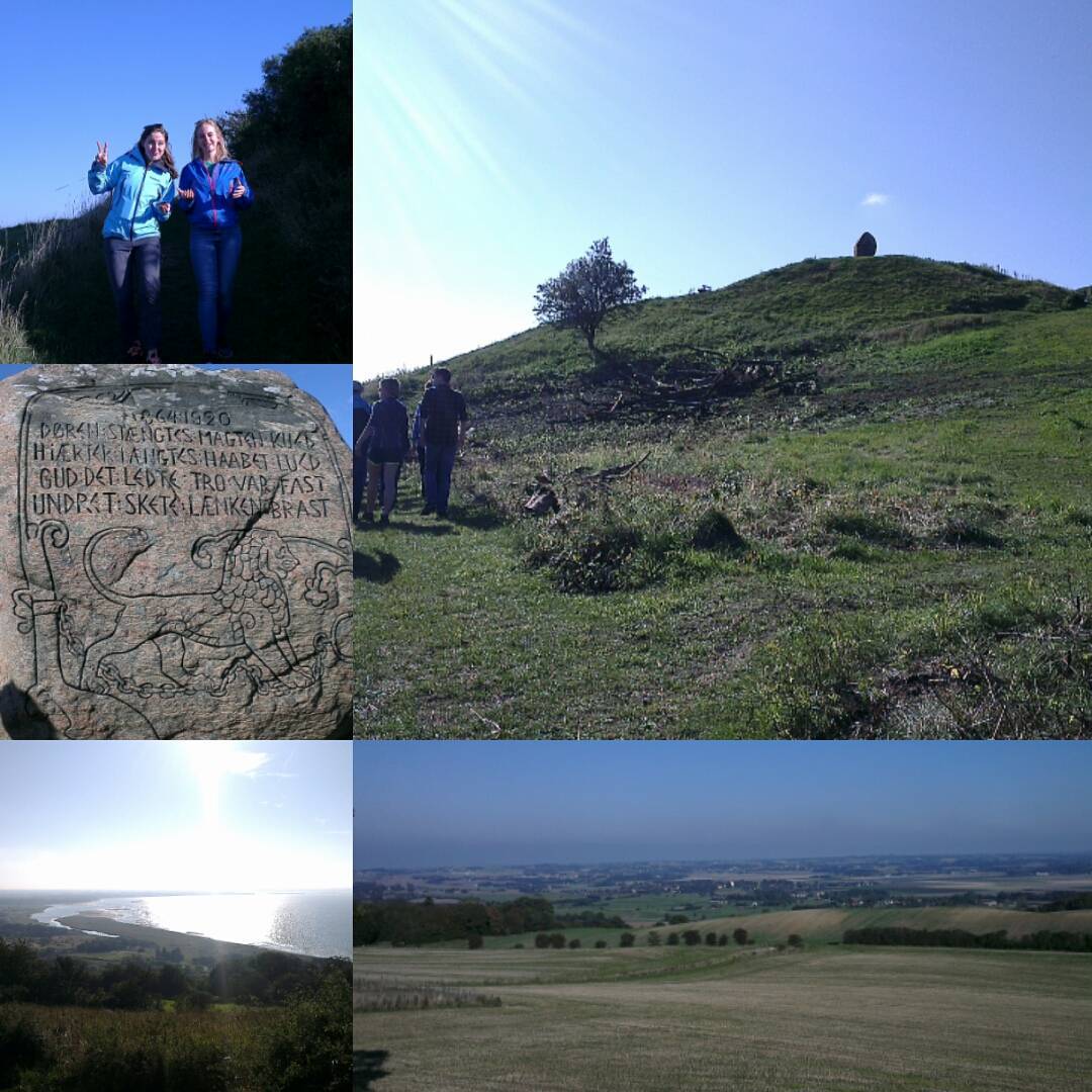
After group work sessions in the morning we went on a field trip to the Geopark Odsherred in the afternoon to learn about the regional cultural and geological background of eastern Denmark. The field trip included visits of two barrows from the Stone Age and Bronze Age as well as an easy hike on one of the highest ’mountains’ in Denmark, the 121 m high mound Vejrhøj. The hilly landscape was largely shaped during the last glacial when advancing and retreating glaciers led to the formation of moraines, meltwater outlets and proglacial lakes.
Photo credit:Henning Åkeson
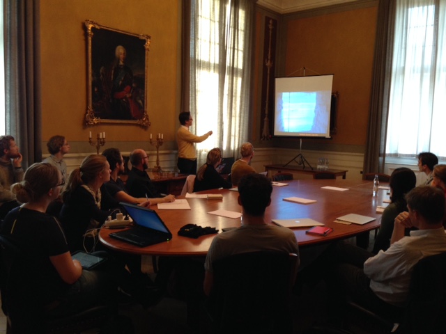
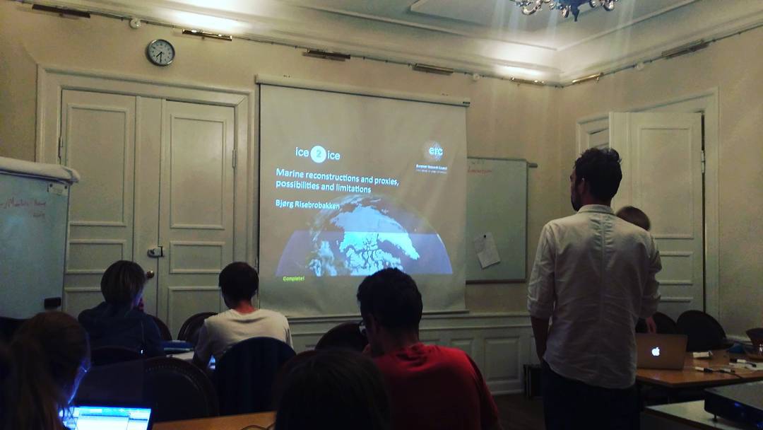
In the evening Bjørg Risebrobakken gave a science talk about proxies in paleoceanography and their possibilities and limitations.
Day 4. Thursday, October 1st
This day was filled with intense group work, preceded by Andreas Born’s talk on the Influence of ice sheet topography and sea ice cover on Eemian Greenland temperature and precipitation.
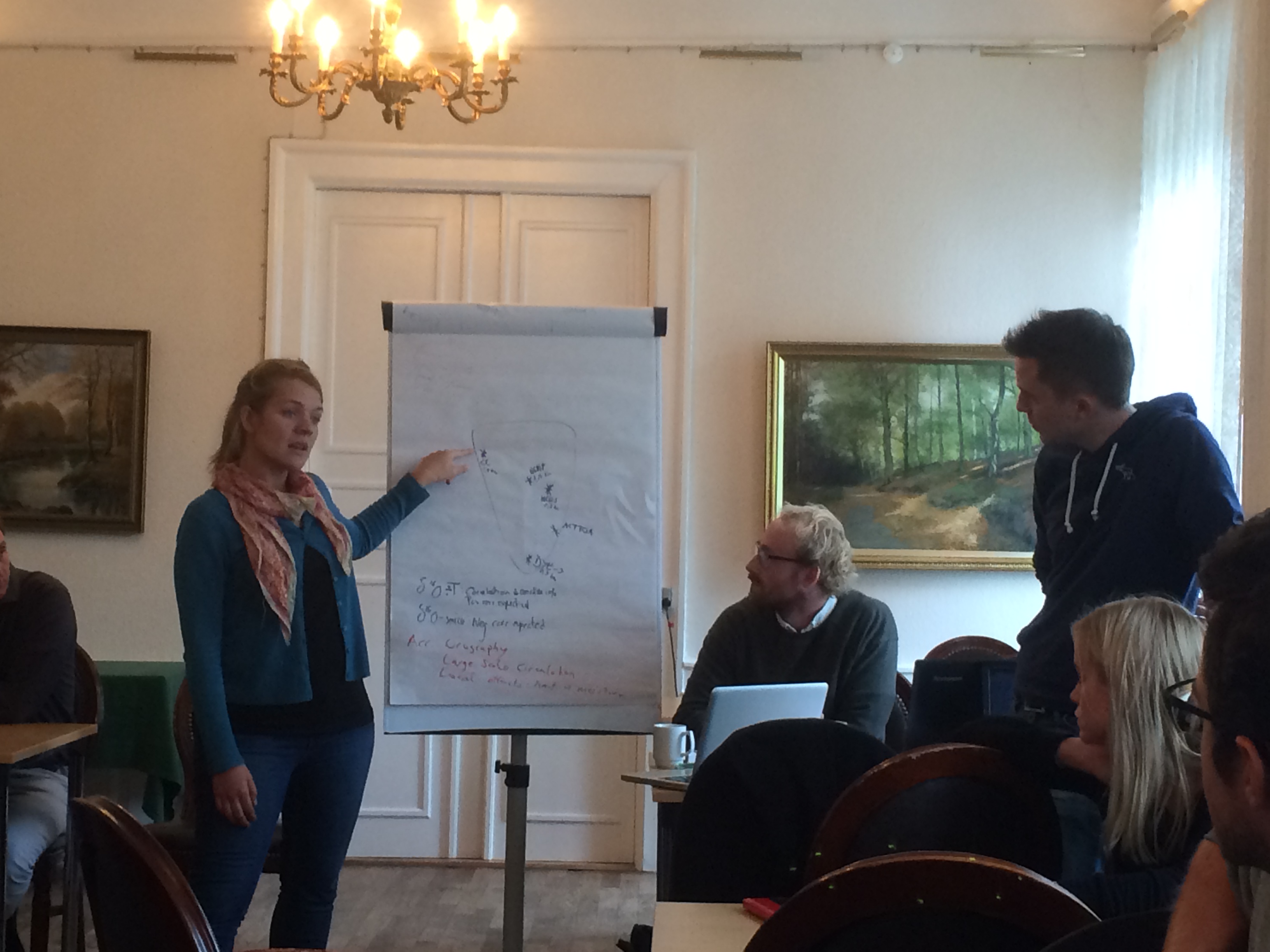
The group work focused on:
Background info on Eemian
Simulations of atmospheric effects on Greenland during Eemian
Precipitation changes (using site of today’s NEEM during Eemian)
Photo credit:Henning Åkeson
Day 5. Friday, October 2nd
The final day involved some intense finalization of the three group projects. Findings were presented after lunch. They main findings were
1) Ocean temperature during Dansgaard–Oeschger (DO) events – The proxy surrogate method has great potential for combining proxy records with model simulations. According to the model runs, the temporal variability of the Nordic Seas and northern North Atlantic can be explained well by the proxy sites available. However, information from eastern Greenland/close to Fram Strait is lacking, and proxy reconstructions from this area would be highly valuable. Spatial maps of sub-surface temperatures from DO event 7, and a constructed idealized DO event, were made. The results were quite sensitive to small changes in the reconstructed sub-surface temperature values. This needs to be investigated further. The results were limited by the little variability in the model run compared to observations.
2) Sea Ice and Greenland accumulation – The correlations patterns between sea ice and accumulation and δ18O data for NEGIS/EGRIP showed that it was difficult to determine the cause of correlations (co-causality problem). The correlation results were not consistent with the NAO pattern driving changes in sea ice and δ18O. However, lower elevation and near-coastal ice cores (Camp Century, Renland, ATC10) were more sensitive to local sea ice conditions.
3) Inverse modeling of ice shelves – Inversion results (for Pine Island Glacier, W. Antarctica) are sensitive to initial guess of the parameter we want to invert for (ice shelf: rheology; grounded ice: basal friction). Form of cost function (absolute/logarithmic/average misfit) renders slightly different results. Also wanted to test how incomplete spatial data coverage affect inversions, but some model technicalities prevented final conclusions here.
The final presentations marked the formal end of the bootcamp. Participants were afterwards witnessing how to skin a deer (hunting season just started the same day) and joined for mushroom picking in the forest nearby. The deer and mushrooms ended up on the grill and in a sauce, and finally on participants’ plates.
Photo credit:Henning Åkeson
Most people thought that the bootcamp was very relevant to their own PhD research, and that they would like to see another such event in the future, in the same or slightly different format.
author: Henning Åkeson on behalf of the ice2ice PhD’s
The 15th Karthaus summer school on Ice Sheets and Glaciers in the Climate System took place from 8th to 19th September 2015 in Karthaus (Bolzano, Italy) on the Italian alps. The course provided knowledges on various aspects of glaciers and ice sheets to Ph.D. students that work on a glaciology-related climate project. Topics included continuum mechanics, kinematics, ice rheology, sliding and hydraulics, numerical modelling, polar meteorology, ice-ocean interaction, ice cores, interaction of ice sheets with the solid earth, glacier fluctuations, and much more-all related to the ice2ice project.
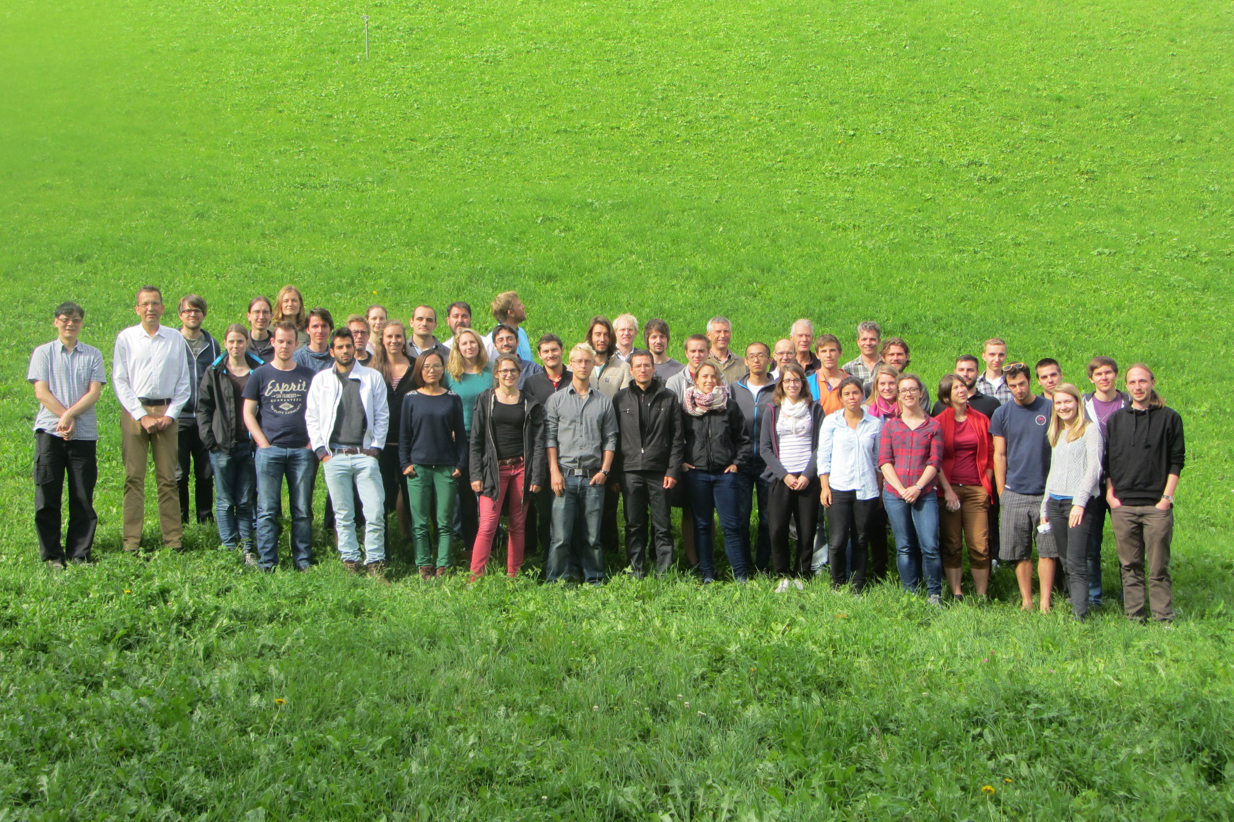
The participants of the 2015 Karthaus Summer
During nearly two weeks, a total of 36 students attended lectures in the morning and exercises in the afternoon. Computer projects, done in groups of three students, was also part of the summerschool programme. The projects were in the end presented to the class. An excursion to the nearby glaciers was also organized, to observe in reality the different aspects of the glacial environment.
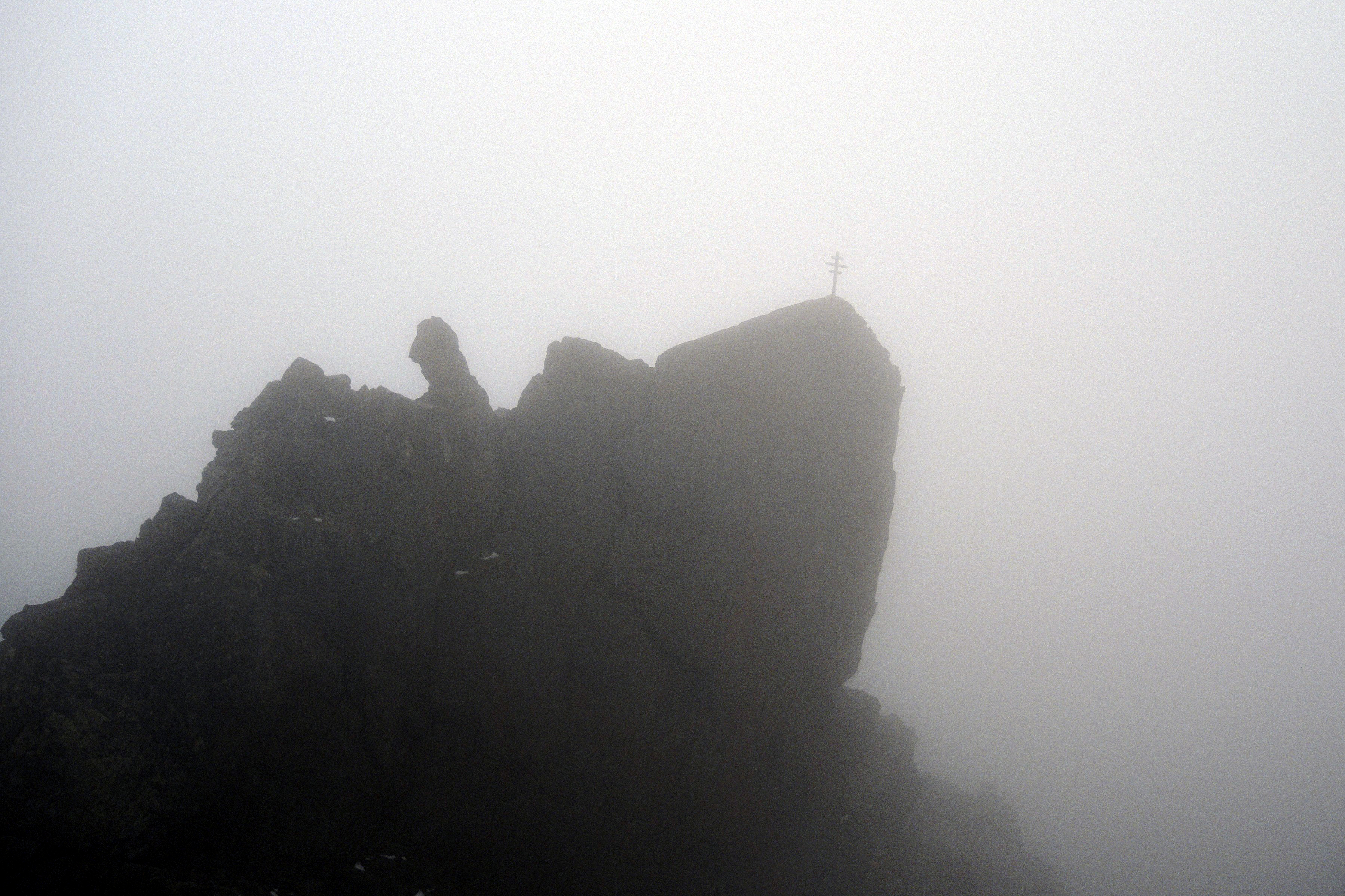
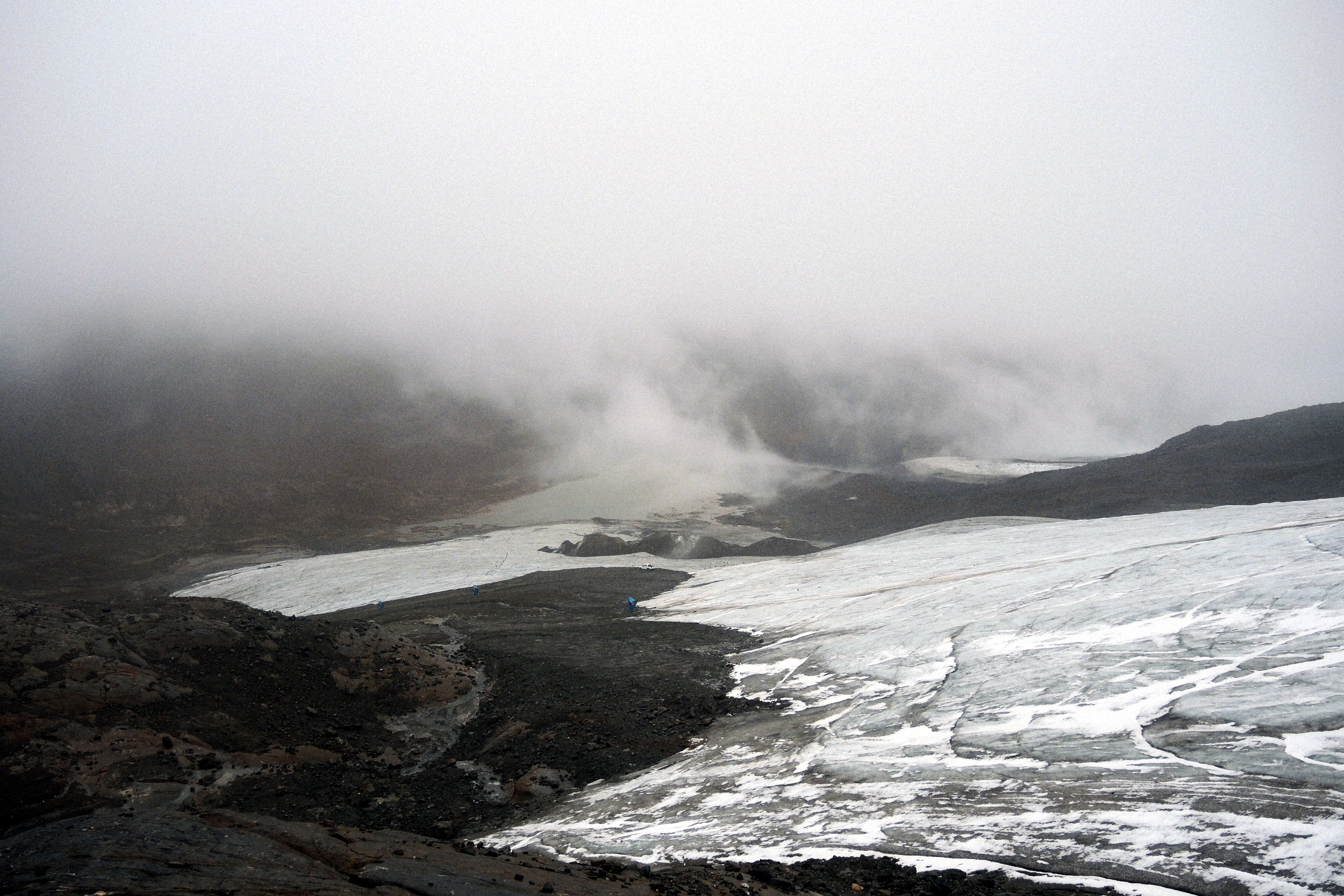
Alpine passes are marked with crosses since the XIII century.Excursion to a nearby glacier
Less than two weeks after arriving the port of Tromsø with G.O. Sars the ice2ice Team Jansen members started the comprehensive sedimentological analyses of the retrieved sediments form the Western Nordic Seas.
Focus are put on two 20 m long piston cores from the shelf outside Scoresbysund and the first results indicate that the selected cores cover ice2ice target intervals: the Eemian interglacial, Marine Isotope Stage 3 and the Holocene.
Our new team member Ida Synnøve Olsen has started sampling and sieving sediments from the mid Scoresbysund transect. Ida is sampling every 5 cm, then sieving and in a microscope picking out foraminiferas (marine plankton with carbonate shells) in order to get a oxygen isotope record.
These cores are currently scanned at the University of Bergen using the X-ray fluorescence (XRF) method. Like on the cruise the team members are working in shifts at the XRF scanner in order to generate as much data as possible within a short time period. That approach will give indications about the elemental composition of the marine sediments and in combination with the existing data from onboard measurements of magnetic susceptibility we are able to develop initial age models for the cores. In which resolution these intervals are resolved in the equivalent cores is currently established by using oxygen isotope stratigraphy and radiocarbon based age determination.
Over the next few weeks the PhD students Evangeline and Henrik, as well as Ashley (Fulbright student) and the new Ice2ice master student Ida will be working in the sediment lab sampling the two piston cores. Sampling will be done at 5 cm intervals in 1/2 cm slices. These will be weighed, dried and sieved before being picked for various foraminifera to conduct isotope analysis. The analysis will help us construct past temperatures and help us to determine the age of the core when compared with isotope concentrations from ice cores. When the MIS3, and DO events are “located” in the core, we will sample the rest of the core in that time frame to conduct other multi-proxy analysis such as Mg/Ca on benthic foraminifera to capture past bottom water temperatures.
In addition to the lab work Henrik is currently working on a high-resolution sea ice record based on biomarkers in core MD99-2284 from the southern Norwegian Sea, which will cover at least two D-O cycles around DO 8 and 7. After having the first age models for our new cores, he will start to generate similar sea ice records for cores from the northern Denmark Strait and the East Greenland margin.
In-depth studies of tephra are conducted by Sarah and scheduled later this autumn. She is currently exploring how to utilize the Flow-cam at the new Earth Lab hosted by Dept. of Earth Science at UoB in order to establish a tephracronology in the Scoresbysund cores.
Want to know what is behind the numbers and curves?
The lab work is a crucial part of the ice2ice project providing us with the basis for our paleoclimatic reconstructions. All Ice2ice members are welcome to join or visit us at our laboratories for a day, a week or a month! Contact Jørund Strømsøe.
The Past 4 weeks a large part of the ice2ice members at University of Copenhagen have spend their time in a freezer in Bremerhaven. They have cut the, in total 586 m long, Renland ice core into smaller samples to prepare for the investigation of the climate signal kept within. Samples for water isotopes, which inform on the past temperature, were made for each 55 cm (1064 samples) and also for each 2.5 cm (>23000 samples). Pieces were cut out for the analysis of greenhouse gases, for the analysis of chemical impurities and also a section for analysis of physical properties, such as crystal structure was cut.
8 persons involved in the ice2ice project from University of Copenhagen participated in the work, which took place at -20C.
The cutting was finished Friday the 11th of September 2015. Now the sections are on the way to leading laboratories around the world for high class analysis to be started in October.
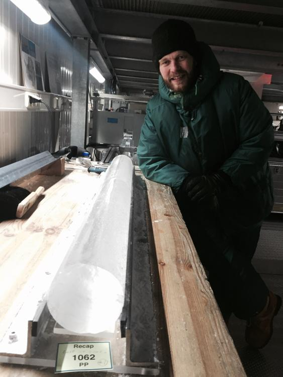
Bo Vinther (Primary Investigator UCPH) with the deepest part of the Renland ice core, which is more than 110.000 years old.
Ice2ice researchers Hannah Kleppin and Markus Jochum has published together with coworkers from Colorado a paper titled “Stochastic Atmospheric Forcing as a Cause of Greenland Climate Transitions” in Journal of Climate. The abstract is presented below and the full article can be found here.
Abstract
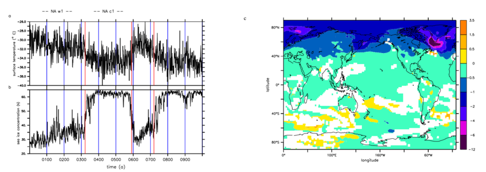
An unforced simulation of the Community Climate System Model 4 (CCSM4) is found to have Greenland warming and cooling events that resemble Dansgaard-Oeschger-cycles in pattern and magnitude (Figure 1a). With the caveat that only 3 transitions were available to be analyzed, we find that the transitions are triggered by stochastic atmospheric forcing. The atmospheric anomalies change the strength of the North Atlantic subpolar gyre, leading to a change in Labrador Sea sea-ice concentration (Figure 1b) and meridional heat transport. The changed climate state is maintained over centuries through the feedback between sea-ice and sea-level pressure in the North Atlantic. We discuss indications that the initial atmospheric pressure anomalies are preceded by precipitation anomalies in the West Pacific warm pool. The full evolution of the anomalous climate state depends crucially on the climatic background state.
Figure 1: (a) Greenland annual minimum surface temperature [◦C] averaged from 55 ◦ to 15 ◦W and 65◦ to 80◦N. (b) Annual maximum of sea ice concentration in the LS (53 ◦ to 65 ◦N to 60◦ to 45 ◦W). The different phases of interest are indicated on top, NA_w1 is the period from year 50 to year 250 and NA_c1 from year 350 to 550. The transition between different warm and cold phases, based on Greenland temperature changes, are marked by red horizontal lines. (c) Surface temperature difference between years 350 and 550 (NA_c1) and 50 and 250 (NA_w1). Regions are only shaded if correlation with Greenland surface temperature (averaged over the same region as in (a)) for the period between year 270 and 470 is significant on a 95 %-level.
The climate modelling part of ice2ice had a very productive meeting in Copenhagen in September with an opportunity to both hear about progress in the simulations and discuss problems, potential pitfalls and the potential results. The science part of the programme commenced with a good overview of the representation of sea ice in CMIP5 models and how this is likely to change presented by Shuting Yang. These results showed that even in a 2°C world, Arctic sea ice is likely to be gone in September. We also considered the EC-Earth – PISM results for the extended RCP8.5 scenario. Shuting showed a linear relationship between sea ice and surface mass balance in this run and there was much discussion on the implications of Arctic ocean stratification and salinity in the models and how this anaylsis can be both used for ice2ice and extended with other models, output and datasets.
Mats Bentsen gave an interesting overview of the NorESM model, the updates since CMIP5 that will be used in CMIP6 and the configuration for the palaeo-simulations. The run-time is impressive and there has been a significant improvement in model performance in the North Atlantic.
Rasmus Pedersen presented a detailed overview of his PhD work using the CESM model to identify the atmospheric response to regional sea ice change, where sensitivity experiments in different sectors of the Arctic Ocean were carried out, with some rigorous questioning afterwards, which he acquitted well.
Peter Langen presented some statistical work on the CMIP5 model outputs and ways to better define uncertainties in projections which is relevant for the way we will analyse the ice2ice datasets.
We also managed to set up some remote participation with Norwegian colleagues not able to join us; Lu Li updated us from Bergen on the challenges and progress in setting up WRF to model the Greenland domain. A couple of issues were identified and the future strategy for both regional models (WRF and HIRHAM5) was firmed up.
Finally there was a wide-ranging discussion session that dealt with coordination of the modelling programme, the planned palaeo-runs and sensitivity experiments and how to synthesise the data and analysis together.