Next week several ice2ice scientists will head towards Vienna. You might wonder why?
The EGU general assembly 2016 will bring together geoscientists from all over the world to one meeting covering all disciplines of the Earth, planetary and space sciences. The EGU aims to provide a forum where scientists, especially early career researchers, can present their work and discuss their ideas with experts in all fields of geoscience.
Thus it is an ideal place for the ice2ice group to discuss new results from both the ReCAP ice core, the sediment cores taken during this years cruise as well as to engange in discussions about recent model runs of both past and present. Below an update of presentations at EGU2016 by ice2ice scientists sorted by day and what kind of presentation.
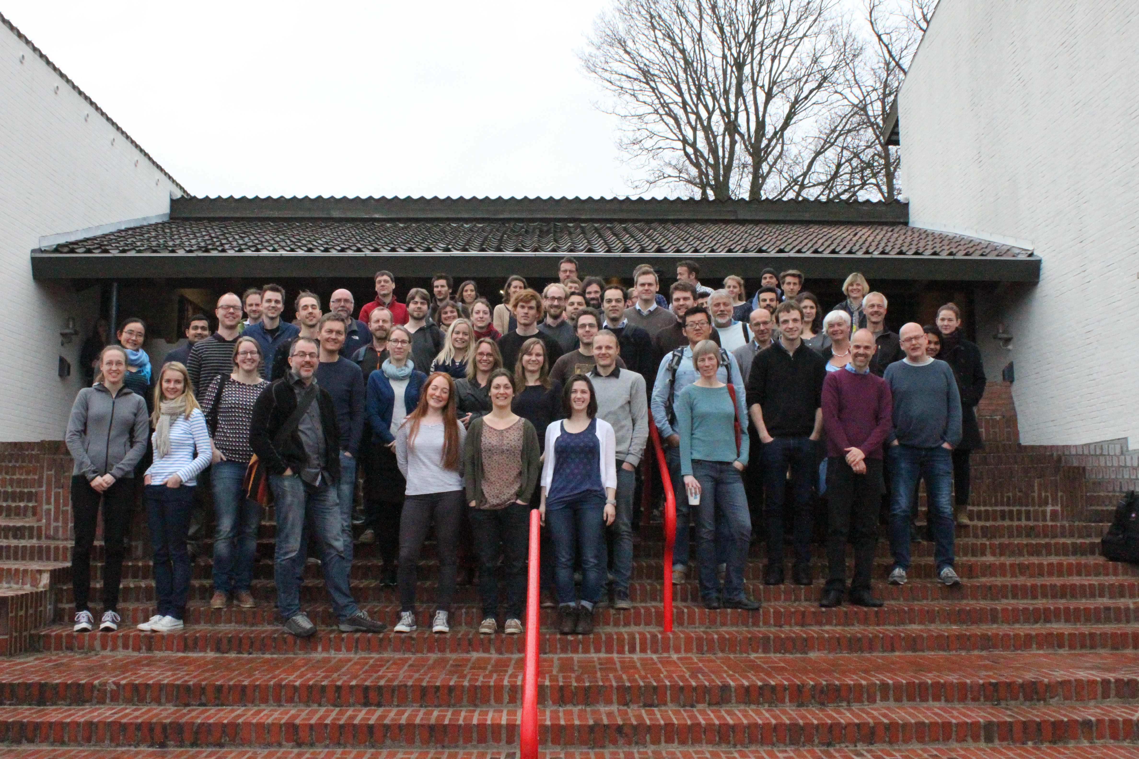
The annual all staff meeting was held in Helsingor in April. With almost 70 participants including internal and external experts and almost the entire Ice2Ice team; ice cores, modelling, sea ice and marine records where discussed day and night.
The annual all staff meeting was held in Denmark, Helsingor surrounded by both forest and ocean and good opportunities for “walk and talks”. The meeting was split into a presentation part and a part of discussing future plans.
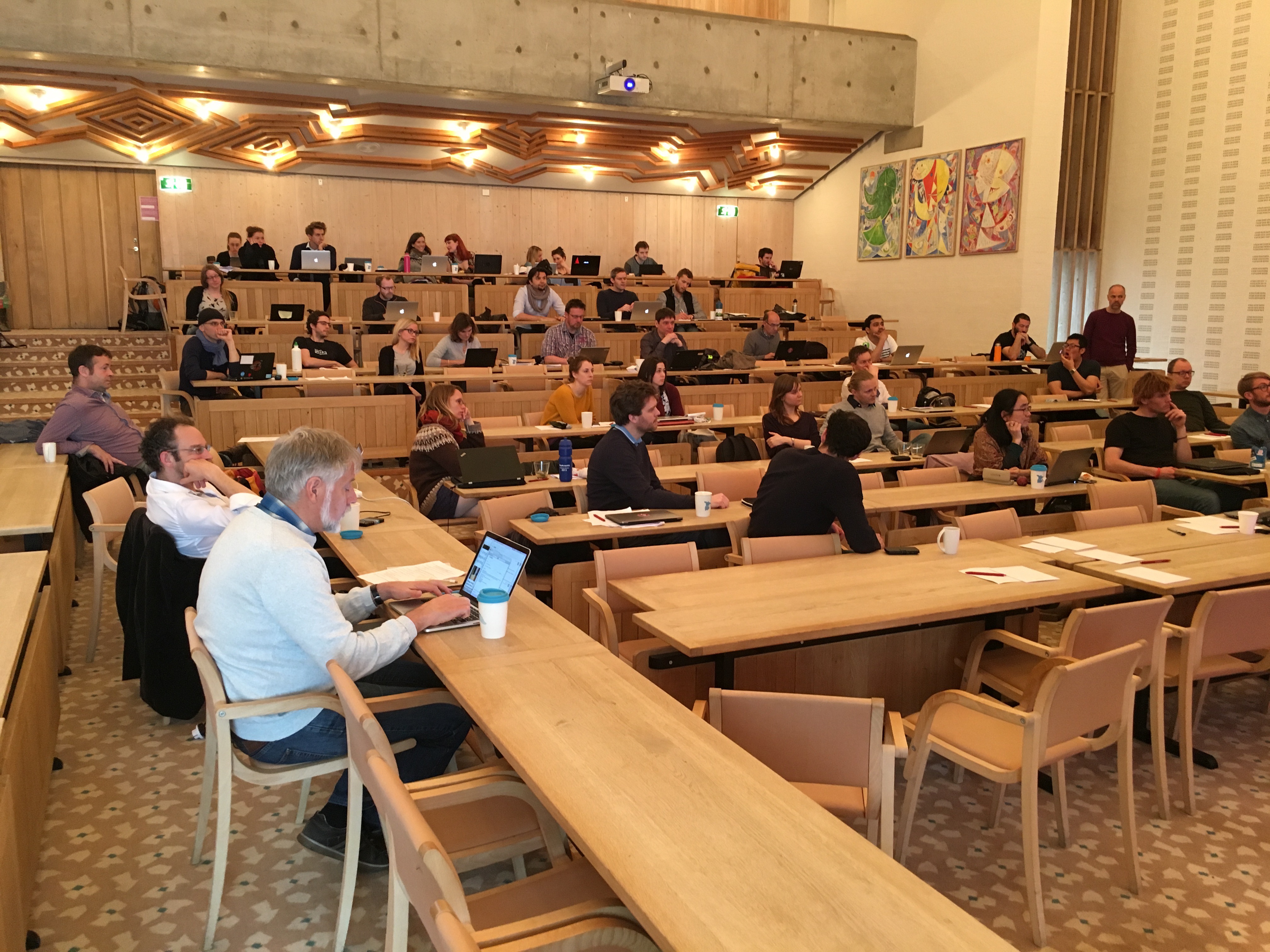
The presentations were kept short to make sure that everybody within the ice2ice community had time to present their work and ideas. The talks were split into the sessions:
Session A – Atmospheric dynamics
Session B – Ice core proxies
Session C – Marine proxies
Session D – Ice Dynamics
Session E -Sea ice/ocean dynamics
Session F – Ocean Dynamics Session
Each session had between 4 and 6 talks by ice2ice members. Further sessions for introducing new people within the ice2ice project, discussing impacts from the more than 5 workshops ice2ice has arranged in the past year, discussion and presentation of past and future field work and more practical info on what to be aware of when travelling between the institutions was presented and discussed.
The second half of the meeting included group discussions, all the work packages (WP1, WP2 and WP3) of the ice2ice project was discussed and a plan including for future meetings, articles and collaboration was made for each work package.
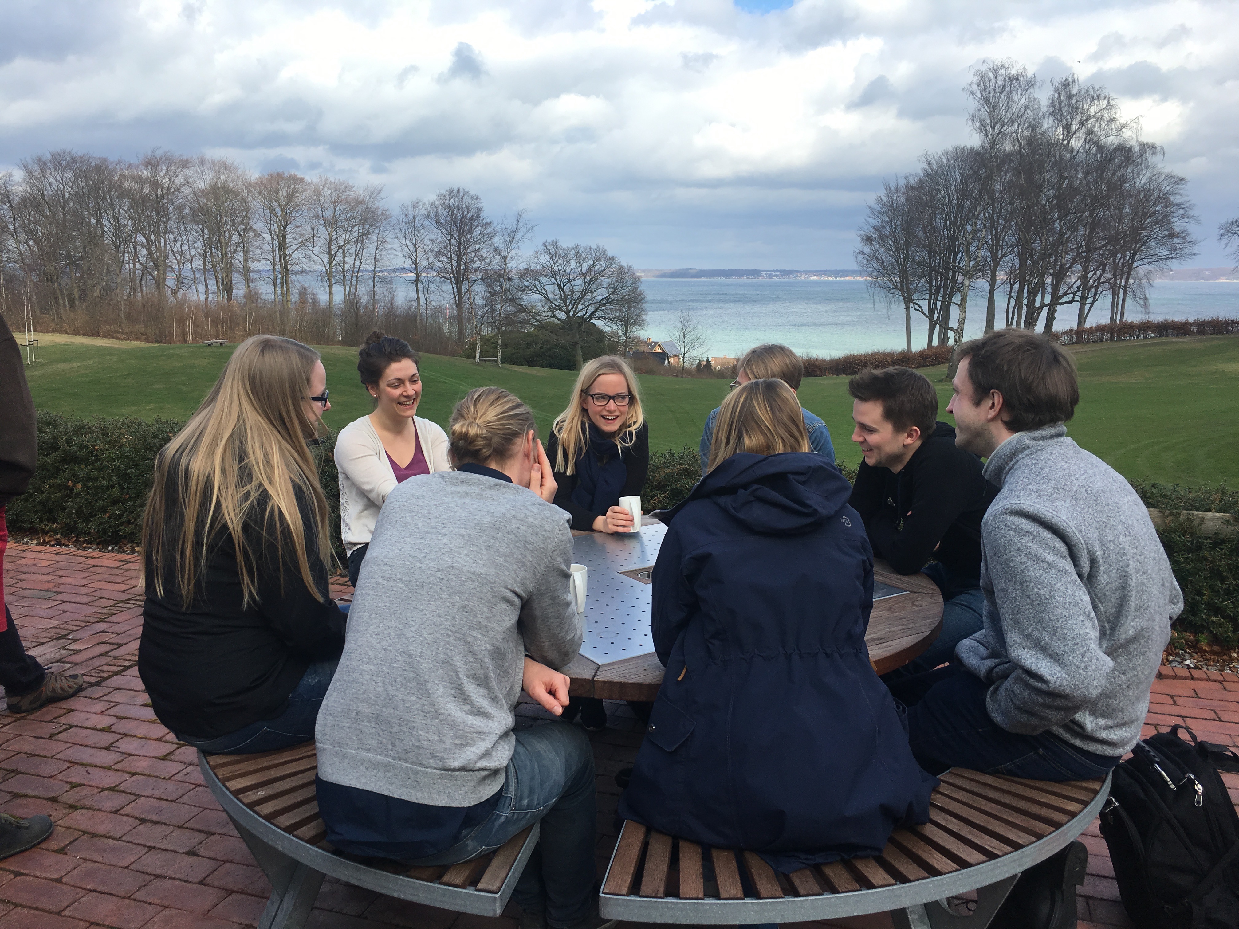
All spare time was used to further discuss collaborative plans between the different institution members.
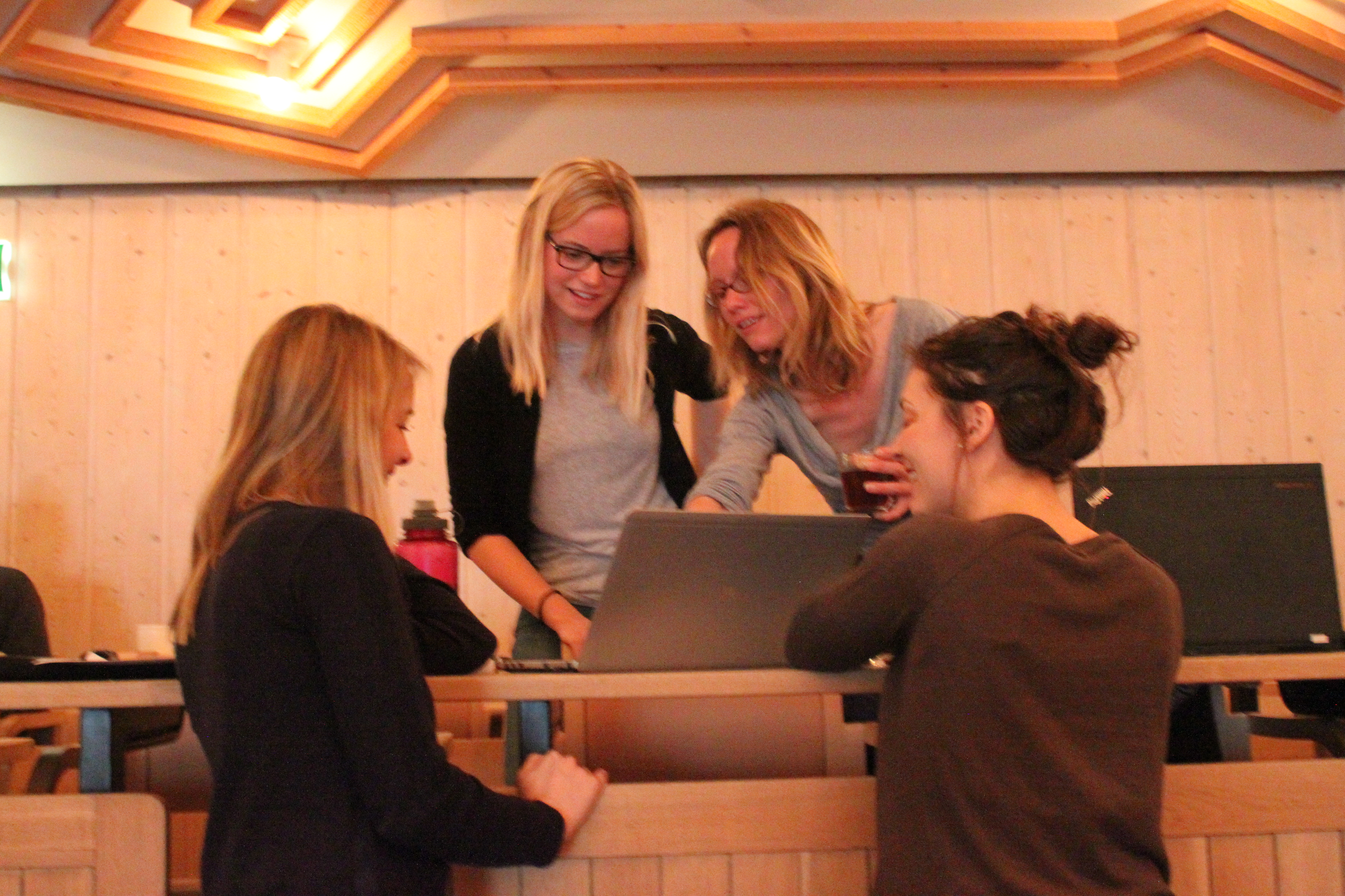
In the breaks all the novel data obtained within the last year was discussed.
During lunch and dinner inter-disciplinary discussions continued between the researchers
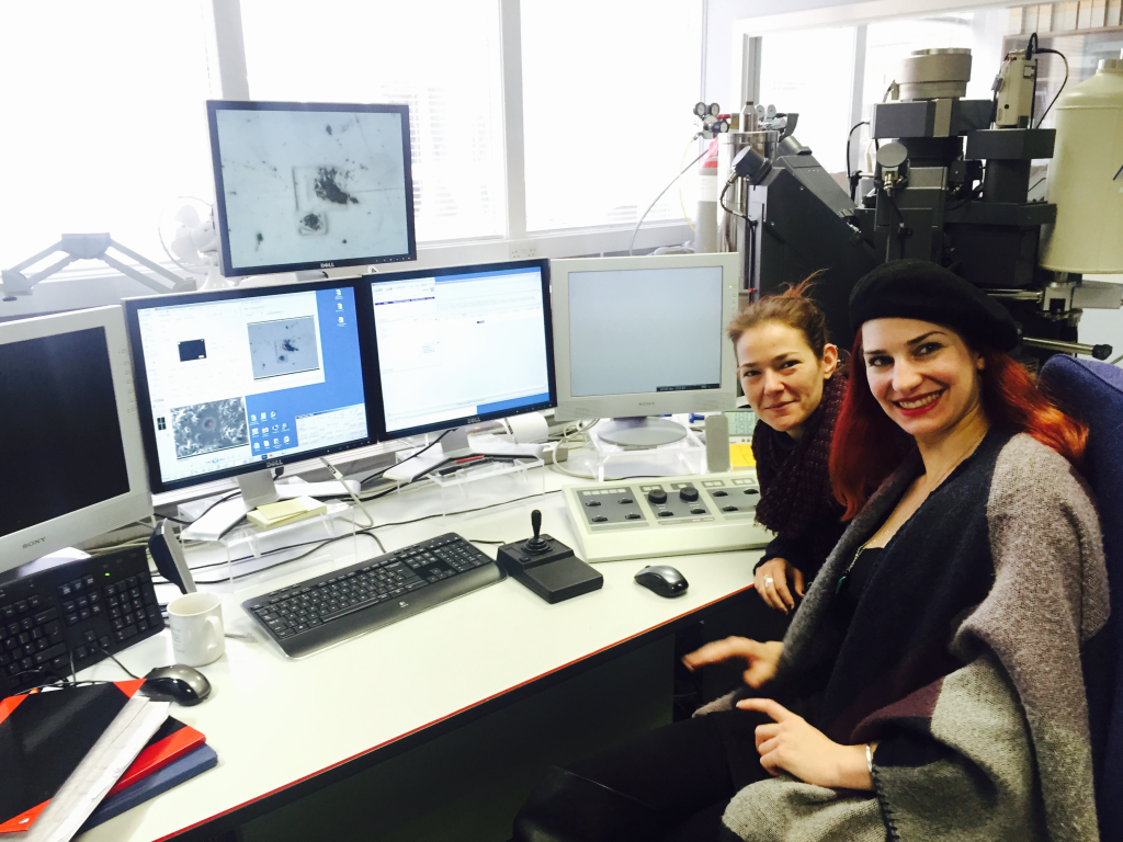
Eliza Cook and Sarah Berben analysing ice core samples by EPMA at Edinburgh.
Five visible tephra layers were identified by naked eye during the processing of the Renland ice core – both in the field and during core cutting at AWI. At the Centre for Ice and Climate, Eliza Cook was able to take sub-samples from each deposit for geochemical analysis and the results form an initial tephrostratigraphy framework for Renland. This framework will be substantially added to when cryptotephra deposits are searched for and identified over the next few months (cryptotephra deposits contain tephra grains in low concentrations and are not visible to naked eye).
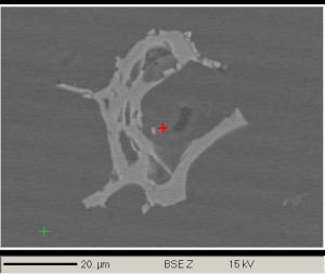
Back-scatter electron image of rhyolitic tephra grain from Dye3
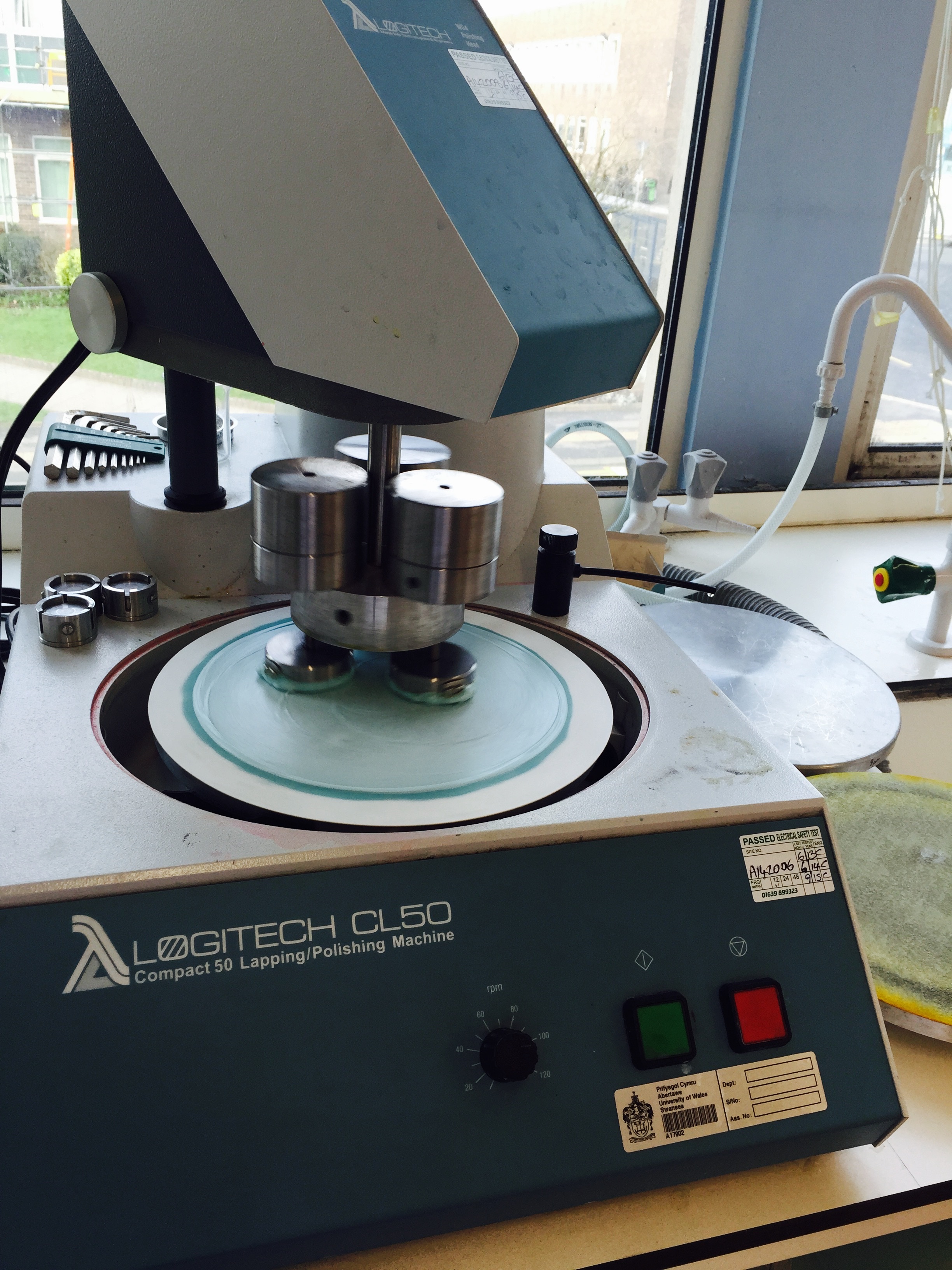
The visible samples were mounted on microscope slides and set in epoxy resin. Once each was confirmed as tephra (and not dust) through optical properties under cross polarised and normal transmitted light, the slides were carefully polished in preparation for geochemical analysis, using 1, 6 and 9 µm diamond suspension polish, to expose a flat, cross section through tephra grains on the microscope slide (pictured). Deriving the major element content from individual tephra shards is facilitated using electron probe micro-analysis (EPMA). Expressed as oxide percentages, up to 13 major elements can be assayed using this approach, including Si, Al, Ti, Fe, Mn, Mg, Ca, Na, K and P, which comprise the non-volatile elements. The EPMA technique uses x-rays to determine the presence and concentration of major elements within individual tephra grains and the technique works on the basis that when a glass shard is ‘bombarded’ with a focussed electron beam, the x-rays generated have a distinct energy and wavelength characteristic of a particular element. Thus, by measuring the intensity of the x-ray signal, an inference can be made as to the abundance of that particular element as the signal generated is directly proportional to the abundance of the element within the shard.
Taking the first samples for EPMA analysis at the Tephra Analysis Unit (University of Edinburgh) in late February provided a good opportunity for Ice2Ice colleague Sarah Berben (from University of Bergen, pictured) to become familiar with Cameca SX100 microprobe, before analysing her own marine tephra samples over the next few months. Over the next couple of years Eliza and Sarah will work together to try to find common tephra deposits in the ice and marine records.
Using a polishing machine with diamond suspension to achieve a clean cross section through individual tephra grains on the microscope slide
In addition to the Renland samples, other Holocene tephra deposits from Dye3 and NGRIP ice cores were also processed during the week, and the results will contribute to improving the Holocene tephrostratigraphy in Greenland and will also contribute to Ice2Ice.
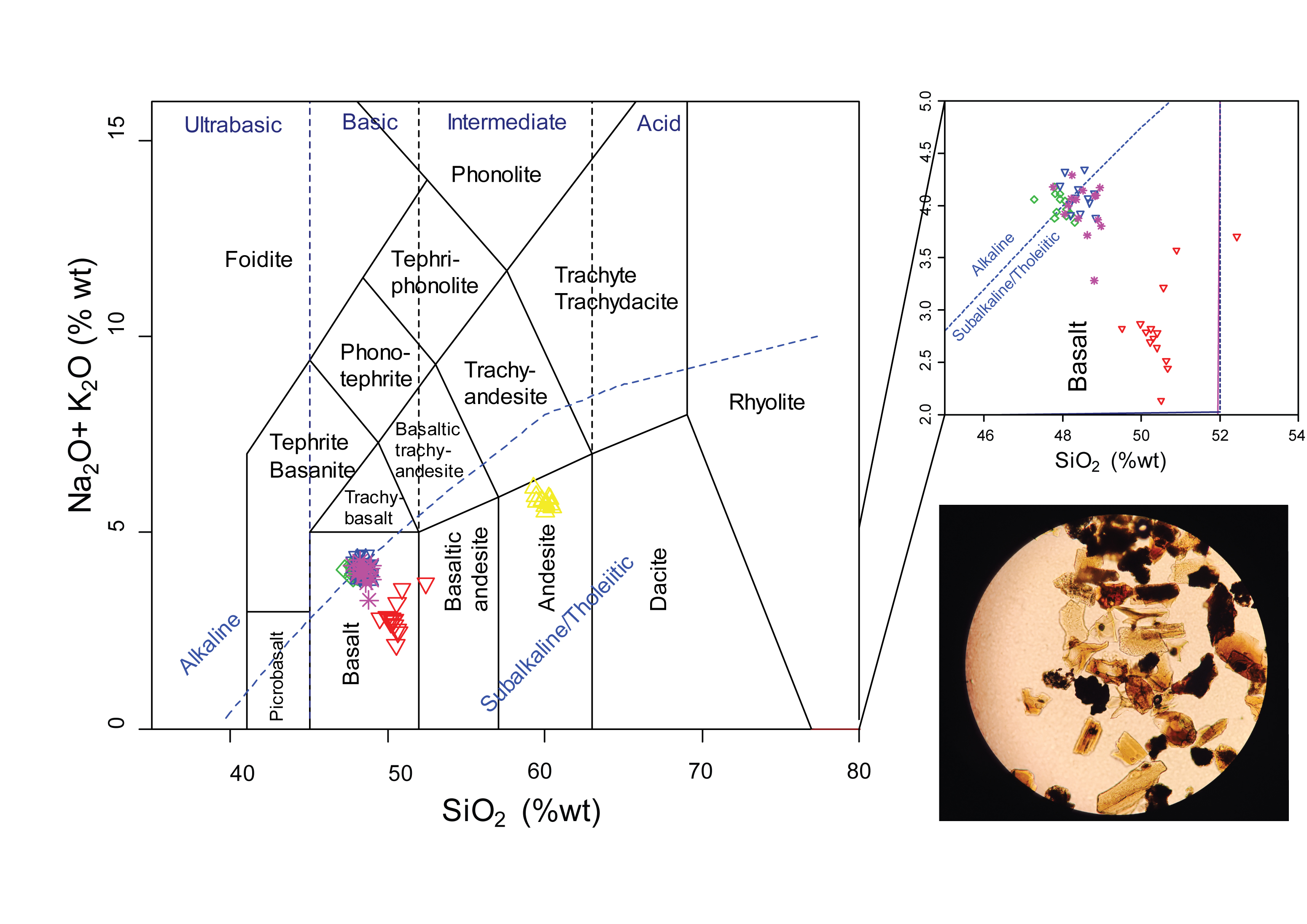
In summary, analysis reveals all tephra deposits to be of Icelandic origin and can be separated into three rock types; Andesite, Tholeiitic Basalt and Transitional Alkali Basalt. This is shown on the total alkali vs silica (TAS) classification diagram, used to discriminate between rock types, based on Na2O+K2O vs SiO2 content. This plot assigns a rock type to samples and is also used to discriminate between alkaline and sub-alkaline products.
ANDESITE A single andesite deposit, has a homogeneous andesite composition, characteristic of products from Hekla, from the Eastern Volcanic Zone of Iceland. Icelandic andesite less than other volcanic products and will form a useful marker deposit.
THOLEIITIC BASALT DEPOSITS There were two tholeiitic basalt deposits. The first has a heterogeneous tholeiitic basalt composition, with two populations, indicating different volcanic sources. The first population has a geochemical similarity to products from Bárdarbunga-Veidivötn and Grímsvötn centres, while the second has a similarity to products from Grímsvötn and Kverkfjöll
Total alkali vs silica plot to discriminate between rock types for Renland visible layers
My recent paper in Geophysical Research Letters (co-led with Torge Martin from Kiel) was in part inspired by discussions at the ice2ice supported ‘MIS3/Southern Ocean and Bipolar Seesaw Workshop’ held in Bergen in January 2015. Check out the paper for the details; read on for a little story telling.
Dansgaard-Oeschger events, in their most iconic form, are saw-toothed 5–16°C temperature variations in Greenland ice cores1,2. Now, more than 30 years after these abrupt climate changes were first seen in the Greenland ice3, we have learned that D-O variability echoes through the entire climate system: in the colour of river sediments in Venezuela4, in water isotope variations in speleothems from China5, in glacial advance and retreat in Patagonia6 and in Antarctic ice cores7, where we see gradual warming of several degrees while Greenland is in the cold (stadial) sate and then gradual cooling periods while Greenland is in the warm (interstadial) state (Fig 1).
Pin the tail on the Donkey
So where does the process start? Palaeoclimatologists have been playing pin the tail on the donkey with DO events for years (I include myself here). This is how you play (thanks Wikepedia11):
“One at a time, each child is blindfolded and handed a paper “tail” with a push pin or thumbtack poked through it. The blindfolded child is then spun around until he or she is disoriented. The child gropes around and tries to pin the tail on the donkey. The game, a group activity, is generally not competitive; “winning” is only of marginal importance.”
Fig 2. Pin the tail on the donkey.
And so we mark our territory. The Laurentide ice sheet bristles with tacks12, as does the North Atlantic13. Clusters of tacks pepper the tropical pacific14, the Nordic seas15 and few decorate Antarctica16 and the Agulhas17. A la mode, the latest are stuck into volcanoes18. Some miss the board entirely19.
So where do we stick the tack with this paper? Well, I’m from Australia and co-author Sune Rasmussen had a sabbatical there and fell in love with the outback and Aussie pies; so naturally we stuck it in the Southern Ocean. Then the reviewers spun us around again and we became less decisive… but first things first, why care about the Southern Ocean during D-Os?
Global sea level20, atmospheric CO2 (ref 21) and (in breaking results from Jeff Severinghuas’ group at SCRIPPS) global ocean heat content22, all vary in phase with the Antarctic temperature trend during D-Os. The fact that these curves look like the Antarctic record does not prove that the southern high latitudes dominate the processes involved in CO2, sea level and total ocean heat content. But the dominance of the Antarctic signal in these rather fundamental measures of the climate state certainly does demand we pay attention to what is going on in the south; if it walks like a duck…
The prevailing explanation for the phasing of the Greenland and Antarctic temperature trends during D-Os is the bipolar ocean seesaw hypothesis23. According to this view D-Os are due to changes in northward ocean heat transport. Increased heat transport is said to cause abrupt warming in the North Atlantic and Greenland (with some help from sea-ice feedbacks) at the same time as gradually depleting the heat reservoir of the Southern Ocean and cooling Antarctica24; vice-versa, weakened northward ocean heat transport is said to cause abrupt cooling in Greenland and gradual warming in the Southern Ocean and Antarctica. This concept works nicely in box models and in many intermediate complexity models25. But it runs into trouble when confronted with a more realistic depiction of the ocean, in which the steeply outcropping isopycnals of the Antarctic Circumpolar Current (ACC) present a barrier to heat transport between the South Atlantic and Southern Ocean. The ACC may not be an insurmountable barrier, but anomalies certainly doesn’t go across nice and easy26.
For additional motivation to look to the south consider that the Southern Ocean currently takes up 75% of anthropogenic heat and 40% of anthropogenic CO2 (ref. 27). Whether the Southern Ocean will continue to provide this service for us is one of the biggest uncertainties in future temperature and sea level rise projections. Understanding what happens in the south during D-O’ seems like a meaningful challenge for the modellers and dynamicists who are trying to predict what the Southern Ocean may do in the future.
Polynyas: windows to the deep ocean
So getting to the point, our GRL paper describes a process that could drive past Antarctic warming events and conceivably even CO2 variations actively from the Southern Ocean itself.
Our idea was inspired in part by microwave satellite data from the 1970’s that shows three consecutive years in which there is a huge ice free area (250,000 km2) in the normally ice-packed Weddell Sea28. The Germans got a ship into this ‘open ocean polynya’ and found that the mixed layer extended to the sea floor29. The sea ice was being kept at bay by massive convective heat loss. The heat supply to sustain the deep convection was supplied by the intermediate depths of the Southern Ocean. The polynya shut down after 1976 and has not reappeared since. However some oceanographers suspect the sort of deep ocean convection that was responsible for the Weddell Polynya may have been more common in the past.
According to Arnold L. Gordon, leader of the original German cruise to the polynya in the 70’s, ocean deep convection may have been the only way for the deep Southern Ocean to vent its heat during the glacial period—because glacial ice cover would have shut down margin processes30. So now we have a potential mechanism to drive Antarctic warming that doesn’t depend on propagating temperature anomalies across the ACC. This was especially attractive to our ‘ACC is a barrier to heat transport’ enthusiast co-author Markus Jochum.
Meanwhile, Torge Martin who I met at U. Washington, while I was a postdoc there, showed me some free-running simulations with the Kiel Climate Model that display some very interesting behaviour in the Southern Ocean. In a 2,000-year free-running simulation, heat accumulates at Southern Ocean intermediate depths and then is released to the atmosphere via deep convection—in the Weddell Sea! The convection lasts until the ocean heat reservoir is depleted, which takes several centuries. Convection then shuts down while the intermediate depths re-accumulate heat. Eventually the threshold of thermal instability is crossed, warm deep water is entrained into the mixed layer, and convection gets off and running again.
Southern Ocean internal variability and Antarctic Warming
In our paper we show that heat loss from the convective zone in the Weddell Sea ultimately causes warming of up to 2°C on the Antarctic continent. Four factors are important (in almost equal measure) in driving the Antarctic warming: ocean to atmosphere heat flux from the convective zone; sea-ice loss and albedo feedback; southward migration of the ACC; and increased heat and moisture transport to Antarctica. The southward migration of the ACC, which takes around 50 years, was a surprise. We put this migration down to heat (i.e. buoyancy) loss from the convective zone dragging the outcropping isopycnals southward. A southward-shifted ACC can also be viewed as a southward shift in the sub-tropical front, which in turn means warmer sea surface temperatures in the mid-latitudes. In response to the mid-latitude warming the atmosphere fluxes more heat toward Antarctica. Fascinating, isn’t it! The behaviour is summed up in our abstract like this:
Simulations with a free-running coupled climate model show that heat release associated with Southern Ocean deep convection variability can drive centennial-scale Antarctic temperature variations of up to 2.0°C. The mechanism involves three steps: Preconditioning: heat accumulates at depth in the Southern Ocean; Convection onset: wind and/or sea-ice changes tip the buoyantly unstable system into the convective state; and Antarctic warming: fast sea-ice—albedo feedbacks (on annual-decadal time scales) and slow Southern Ocean frontal and sea surface temperature adjustments to convective heat release (on multidecadal-century time scales) drive an increase in atmospheric heat and moisture transport toward Antarctica. We discuss the potential of this mechanism to help drive and amplify climate variability as observed in Antarctic ice-core records.
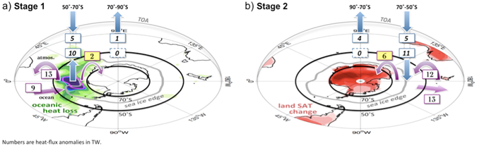
The two-stage response of the southern high latitudes to open ocean deep convection is illustrated in the schematic below (Fig 3.)
Fig 3. Schematic of the annual mean heat flux anomalies during the two-stage Antarctic warming process. (a) Stage 1, active deep convection, with ocean heat loss depicted by green and blue shading, the sea-ice edge in gray, and the 200 m mixed layer depth isoline in magenta (indicating the deep convection area). (b) Stage 2, maximum in Antarctic warming, surface air temperature changes over land depicted by red shading. For both stages vertical blue arrows and boxes give the direction and strength of anomalies in top of atmosphere (TOA) and surface heat fluxes averaged over latitude bands 50–70°S and 70–90°S. Curved purple arrows show the direction and strength of atmospheric zonal mean meridional heat flux anomalies across 50°S and 70°S; horizontal purple arrows show the same for the ocean at 50°S.
Ok, so where’s the link to the north?
As our reviewers pointed out, the mechanism above could be an interesting form of internal climate variability without necessarily having anything to do with D-Os! It’s a good point and I can’t rule out that they are right (yet). So on to some speculation.
Accounting for the time relationship between the Antarctic and Greenland temperature records across the D-O events would call for a process to push the southern high latitude system toward the deep-convecting warming mode while Greenland is in cold stadial conditions (and vice versa). During Greenland stadials we have good evidence that the Inter Tropical Convergence Zone and the Southern Ocean surface wind field are both shifted south5,31. Southward shifted winds would indeed be expected to push the Southern Ocean system toward the convective state by enhancing the Ekman-driven upwelling of intermediate-depth waters, enhancing the advection of sea ice northward away from the convective zone, and deepening the mixed layer32. The situation would be reversed in the case of Greenland interstadials in which there is evidence for a northward shift in the ITCZ and Southern Ocean surface wind field.
Hence we present a chain of coupled ocean and atmosphere processes that would help to bridge the oceanic barrier formed by the ACC. Some things we want to examine next are whether the deep convection events could also release CO2 to the atmosphere and whether the recharge of the heat reservoir that sustains the deep convection events may be linked to the strength or depth of the Atlantic Overturning.
So what about the donkey? Well, at this stage I’m still hanging on to my tack and increasingly of a mind that trying to define where the process starts may not be the most constructive way to tackle the D-O problem. A better approach may be to try to identify the necessary processes and to reject the processes that conflict with the data (e.g. as appears the case with meltwater forcing33) or that conflict with the physics (as may be the case with the bipolar ocean seesaws reliance on propagating anomalies across the ACC). Watch this space.
NGRIP members (2004), High-resolution record of Northern Hemisphere climate extending into the Last Interglacial period, Nature 431, 147.
Kindler, P. et al. (2014), Temperature reconstruction from 10 to 120 kyr b2k from the NGRIP ice core, Clim. Past 10, 887–902.
Dansgaard, W. et al. (1982), New Greenland Deep Ice Core, Science 218 (4579), 1273.
Peterson, L.C. et al. (2000), Rapid Changes in the Hydrologic Cycle of the Tropical Atlantic During the Last Glacial, Science 290, 1947.
Wang, Y. J. et al. (2001), A High-Resolution Absolute-Dated Late Pleistocene Monsoon Record from Hulu Cave, China, Science 294, 2345.
Moreno, P.I. et al. (2009), Renewed glacial activity during the Antarctic Cold Reversal and persistence of cold conditions until 11.5 ka in SW Patagonia, Geology 37, 375.
EPICA Community Members (2006), One-to-one coupling of glacial climate variability in Greenland and Antarctica, Nature 444, 195.
Parrenin, F. et al. (2013), Synchronous change of atmospheric CO2 and Antarctic temperature during the last deglacial warming, Science 339(6123), 1060.
Rasmussen, S. O. et al. (2014), A stratigraphic framework for abrupt climatic changes during the last glacial period based on three synchronized Greenland ice-core records: Refining and extending the INTIMATE event stratigraphy. Quat. Sci. Rev. 106, 14.
WAIS Divide Project Members (2015), Precise interpolar phasing of abrupt climate change during the last ice age, Nature 520, 661
MacAyeal, D.R. (1993), Binge/purge oscillations of the Laurentide Ice Sheet as a cause of the North Atlantic’s Heinrich events, Paleoceanography 8(6), 775.
Broecker, W.S., D.M. Peteet, and D. Rind (1985), Does the ocean-atmosphere system have more than one stable mode of operation? Nature 315, 21.
Kleppin, H. et al. (2015), Stochastic atmospheric forcing as a cause of Greenland climate transitions, J. Clim. 28, 7741.
Dokken, T. M. et al. (2013), Interactions between ocean and sea ice intrinsic to the Nordic Seas, Paleoceanography, 28, 491.
Weaver, A. J. et al. (2003), Meltwater Pulse 1A from Antarctica as a Trigger of the Bølling-Allerød Warm Interval, Science 299, 1709.
Marino, G. et al. (2013), Agulhas salt-leakage oscillations during abrupt climate changes of the Late Pleistocene, Paleoceanography 28, 599.
Baldini, J.U., R.J. Brown & J.N. McElwaine (2015), Was millennial scale climate change during the Last Glacial triggered by explosive volcanism? Nature Scientific Reports, 5:17442.
Braun, H. et al. (2005), Possible solar origin of the 1470-year glacial climate cycle demonstrated in a coupled model, Nature 438, 208.
Siddall, M., E.J. Rohling, W.G. Thompson & C. Waelbroeck (2008), Marine isotope stage 3 sea level fluctuations: Data synthesis and new outlook, Rev. Geophys. 46.
Bereiter, B. et al. (2012), Mode change of millennial CO2 variability during the last glacial cycle associated with a bipolar marine carbon seesaw, Proc. Nat. Acad. of Sci.109(25), 9755.
Bereiter, B. et al. (2016), Mean ocean temperature change over the last transition based on atmospheric changes in heavy noble mixing ratios, International Partnerships in Ice Core Science, Hobart, March 2016.change during the last ice age, Nature 520, 661.
Crowley, T.J. (1992), North Atlantic deep water cools the Southern Hemisphere, Paleoceanography 7, 489.
Stocker, T. F. & S. J. Johnsen (2003), A minimum thermodynamic model for the bipolar seesaw, Paleoceanography 18(4), 1087.
Schmittner, A., O.A. Saenko & A.J. Weaver (2003), Coupling of the hemispheres in observations and simulations of glacial climate change, Quat. Sci. Rev. 22, 659.
Ferrari, R., & M.J. Nikurashin (2010), Suppression of eddy diffusivity across jets in the Southern Ocean, J. Phys. Oceanogr. 40, 1501.
Frölicher, T.L. et al. (2015), Dominance of the Southern Ocean in anthropogenic carbon and heat uptake in CMIP5 models, J. Clim., 28, 862–886, doi:10.1175/JCLI-D-14-00117.1.
Carsey, F. D. (1980), Microwave observation of the Weddell polynya, Mon. Weather Rev. 108, 2032.
Gordon, A.L. (1982), Weddell deep water variability, J. Mar. Res. 40, 199.
Montade, V. et al. (2015), Teleconnection between the Intertropical Convergence Zone and southern westerly winds throughout the last deglaciation, Geology 43(8), 735.
Cheon, W.G., Y.-G. Park, J.R. Toggweiler & S.-K. Lee (2014), The relationship of Weddell polynya and open-ocean deep convection to the southern hemisphere westerlies, J. Phys. Oceanogr., 44, 694.
Barker, S.C. et al. (2015), Icebergs not the trigger for North Atlantic cold events, Nature 520(7547), 333.
Every second month the DMI and NBI groups meet to discuss progress within the ice2ice frame. During these meetings we discuss progress within individual projects, model runs needed, but also more practical issues, such as when next to meet.
Thursday March 17th we had a great meeting with a lot of science discussion. A summary of some of the presented material and project ideas can be found below with a headline for each individual presenter. Besides the four speakers below, Martin Olesen also gave an update on his work.
1420 year long climate change run at DMI by Shuting Yang
A 1400-year long climate change simulation had been performed using the fully coupled climate model-Greenland ice sheet model system, EC-Earth – PISM model at the DMI’s previous HPC system, in order to investigate the evolution of the Greenland ice sheet in a changing climate, and its feedback to the climate system. The long simulation followed the CMIP5 historical and extended RCP8.5 protocol starting from the preindustrial condition at 1850 and spanned to 3269. We examined briefly the characteristics of the climate and the Greenland ice sheet in this long simulation. A number of research topics are suggested and further investigations have been evolved.
Signal transmission in Ocean General Circulation Models
Observations suggest that there exists an anti-phase relationship between the climate of the northern and southern hemisphere during Dansgaard-Oeschger (DO) events. A complete explanation for DO events thus needs to encompass the story of why there is an inter hemispheric climate response. One way to assess the physics is through experiments using General Circulation Models (GCM), but this approach relies on that the model in use is able to resolve the waves that convey the climate signal. The ocean in particular is believed to play a role in the process of transmitting the signal through Kelvin and Rossby waves. The figure displays the model results from a simple shallow-water model in a domain that is thought to represent the equatorial region of the abyssal Atlantic Basin. It is seen how a Kelvin wave is travelling eastward along the equator, setting up the deep circulation. It is the desire to project these results from a simple model onto a more complex ocean GCM.
Propagation of ocean waves in a simple shallow water model of the equatorial Atlantic
What is driving the mass flux variability at the NEGIS outlets.
The dynamic mass loss from marine terminating outlet glaciers is a significant contribution to the current mass budget of the Greenland ice sheet. Using the Uá shallow shelf approximation model together with new ESA CCI GIS surface velocity maps, thisstudy presents initial results on the current seasonal variations of basal properties of the marine outlets of the Northeast Greenland ice stream, one of which recently has been found to exhibit an accelerated retreat since 2012. Furthermore, the groundwork is laid out for future work on correlating such changes with climatic parameters and determining possible impacts on the up-stream catchment area.
Flow patterns for the area around the NEGIS outlet glaciers.
As part of Danish Arctic activities in the Arctic, scientific observations and modeling estimates of various kind are provided to the interested public under www.PolarPortal.dk. As a new effort the Danish Meteorological Institute plans to use the in-house high resolution weather forecast model of the Greenlandic territory to drive the Permafrost model GIPL with the computed atmospheric information. The permafrost model is used in a close collaboration with the Geophysical Institute Permafrost Laboratory (LINK for the Institute name: http://permafrost.gi.alaska.edu/about) in Fairbanks, Alaska, USA.
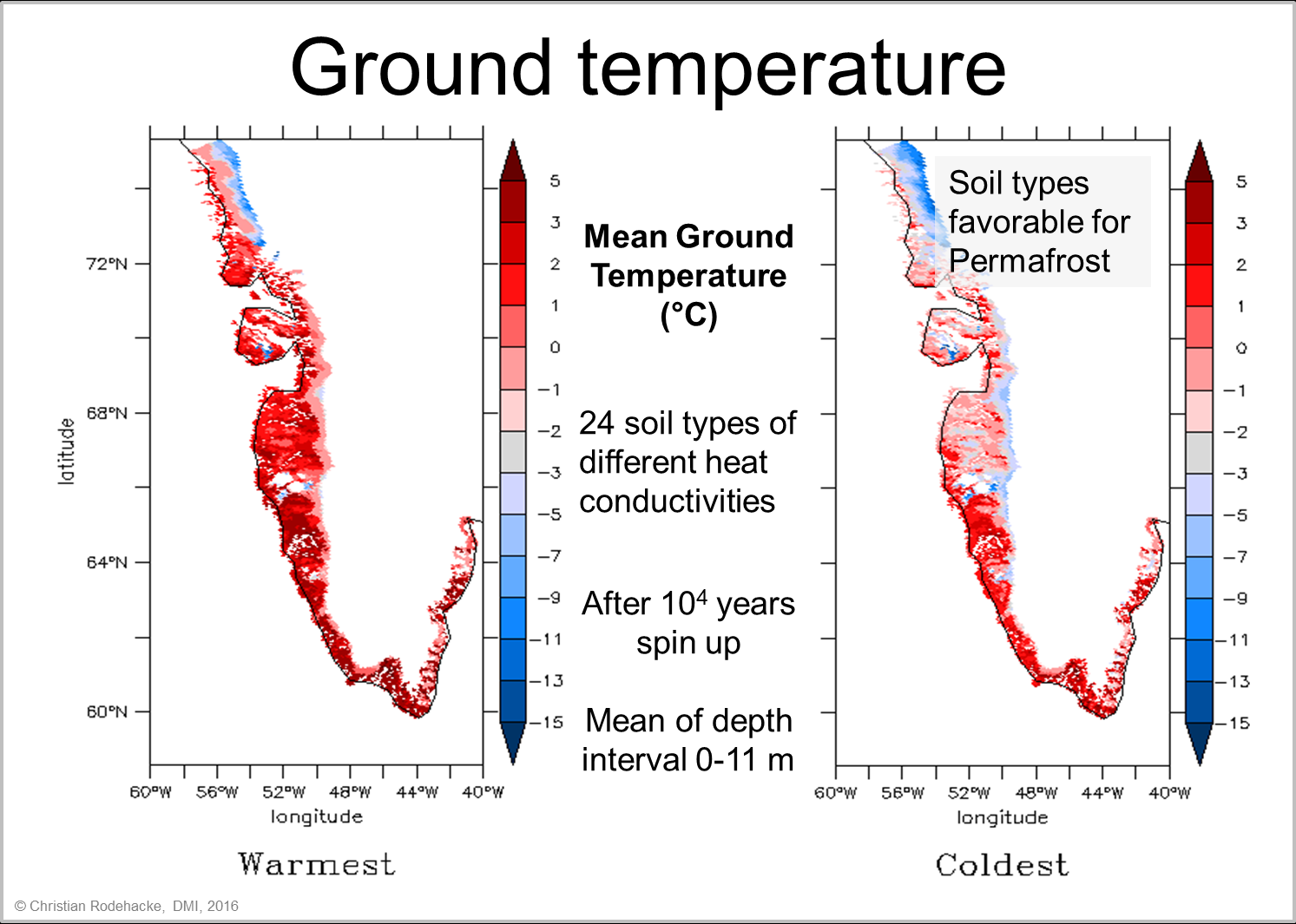
As an initial study we simulate the ground temperature in the southwest part of Greenland. At each grid location we consider 24 different soil profiles that differ in the layering of soil texture, soil material, pore space, water content, and thermal properties. These ground properties determine strongly the heat flow in the ground and, ultimately if permafrost is present. The figure shows the distribution of the computed mean ground temperature in the upper 11 meters in red-blue colors (see colorbar) while the black line follows approximately the coast. The left subfigure depicts the ground temperature where the ground properties generate maximal temperature at of each grid point; the ground properties support a warm ground. The right subfigure shows instead the corresponding minimal temperature in the ensemble of 24 soil types. In this case the layering of ground properties favor permafrost conditions. This example highlights both the need to choose adequate soil properties to simulate permafrost conditions, and, for unknown ground conditions, to compute the conditions for various types to delimit the range of expected ground temperatures.
Ground temperature for the Greenland coast line, with the most favorable soil type and least favorable soil type for Permafrost. Credit: Christian Rodehacke
DMI’s Ruth Mottram er en af verdens førende eksperter på gletsjerspalter, som er vigtige for at forstå isens dynamik f.eks. i Grønland. Det er ikke en helt ufarlig profession.
“Jeg glider, falder, slår mit hoved mod isen og bliver kilet fast, så jeg ikke kan røre mig. Til sidst får min assistent halet mig fri. Efter turen på hospitalet ligner jeg en, der har været involveret i en bilulykke”.
Sådan fortæller DMI’s Ruth Mottram om nærkontakt med en såkaldt gletsjerspalte: Dybe sprækker i de store iskapper, der findes på Grønland, Antarktis, Island og i nogle af Jordens store bjergkæder. Sammen med internationale kolleger har hun netop publiceret en artikel, der samler al den tilgængelige viden om spalterne og deres betydning.
Den dybere mening
Men hvorfor det farlige feltarbejde?
“Jeg er en af de få i verden, der reelt har forsøgt at måle dybden af gletsjerspalter”, siger Ruth Mottram. Og hun gør det ikke for sjov. Viden om spalterne er kritisk for at forstå, hvordan isen opfører sig, hvordan den bevæger sig, smelter, kollapser og ender som isbjerge.
Ruth Mottram har blandt andet sandsynliggjort, at spalterne ikke dannes fra overfladen og ned, men starter i dybden og arbejder sig opad. Hun har også været med til at påvise, at spalterne er vigtigere for iskappernes massebalance end hidtil antaget. Massebalancen er forholdet mellem isdannelse gennem snefald og komprimering og så kælvning af isbjerge og smeltning.
“Tæt på overfladen virker spalterne som solfangere. De påvirker også turbulensen i luftmassen, der blæser hen over isen. Begge dele er med til at øge afsmeltningen”, forklarer hun.
Spalterne er også vigtige kanaler for smeltevand. Det gør dem endnu farligere for forskerne og fører til fænomenetkryo-hydrologisk opvarmning.
“Det er et klodset ord”, griner hun. “Det betyder bare, at da vandet er varmere end isen, så transporterer spalterne i praksis energi ned i gletsjeren, som dermed smelter indefra”.
Spalterne er kritiske for at forstå, hvordan gletsjeren virker. Her et ti processer, hvor de indgår: (1) Isen optager solenergi mere effektivt, (2) luften, der flyder over den ujævne is, bliver mere turbulent (3) spalter, der lukker, fanger kold luft og sænker isens temperatur, (4) den nedre dele af gletsjeren bliver mere porøs, og mere vand bliver fanget nær overfladen af isen, (5) den øvre del af gletsjeren slipper hurtigere af med smeltevand, (6) søer nede i gletsjeren dræner hurtigere, (7) større variationer i nedsivningen af vand og samlet set langsommere gletsjerbevægelse, (8) forøget kryo-hydrologisk opvarmning, (9) forøget hydrologisk svækkelse af isen, og (10) kælvning af isbjerge.
Sådan ser man ud tre dage efter en tur i en gletsjerspalte. Ruth Mottram ser frem til, at ny teknologi kan gøre udforskningen en smule mindre farlig. Klik for stor version.
Vigtige for modellerne
De såkaldte flydemodeller for iskapperne, der beskriver isens bevægelser, er blevet meget bedre de senere år. Men der mangler fortsat vigtige elementer.
“Kun få modeller indeholder beskrivelser af gletsjerspalter eller de processer i isen, som de sætter i gang”, siger Ruth Mottram. Det er hun og danske kolleger i ERC-projektetice2icedog godt i gang med at råde bod på ved at forbedre DMI’s flydemodel, så den blandt andet beskriver kælvning ud fra hendes forskning i gletsjerspalter.
“Vores job er at matematiske beskrive de komplicerede processer så simpelt, at de kan indarbejdes i modeller, der dækker hele Grønland. Jo bedre modellerne er, jo bedre kan vi forudsige, hvor hurtigt isen kan og vil ændre sig og dermed få bedre styr på, hvor meget Indlandsisen f.eks. bidrager til ændringer i det globale havniveau nu og i fremtiden”.
Forskerholdet bag den nye artikel håber, at den fører til mere forskning på området – og til at flere isforskere får øjnene op for, hvor vigtige spalterne er for at forstå iskappernes dynamik. Ruth Mottram håber personligt på, at ny teknologi fremover vil gøre arbejdet mere sikkert, så det næste gang er en drone – og ikke hende selv – der får et par på hovedet.
Reference og kontakt
Colgan, W., H. Rajaram, W. Abdalati, C. McCutchan, R. Mottram, M. S. Moussavi, and S. Grigsby (2016), Glacier crevasses: Observations, models, and mass balance implications, Rev. Geophys., 54, doi:10.1002/2015RG000504.
For pdf af artiklen og for kontakt til Ruth Mottram skriv tilkommunikation@dmi.dk
One of the goals of ice2ice is to reconstruct the history of Arctic sea ice from Greenland ice core records. Ice core scientists currently have two methods for doing this (sodium and Methanesulphonic acid, MSA) although in collaboration with colleagues in Italy (University of Venice) and Australia (Australian Antarctic Division, AAD) we are working on a third sea ice proxy: halogens.
The halogen elements (Fluorine, Bromine, Chlorine, Iodine) are highly reactive and happen to be key elements in chemical reactions that take place on the sea ice surface. Understanding the link between sea ice, halogen chemical reactions and ice cores requires that we take samples from a variety of locations, covering the range of variability in sea ice and snow deposition conditions.
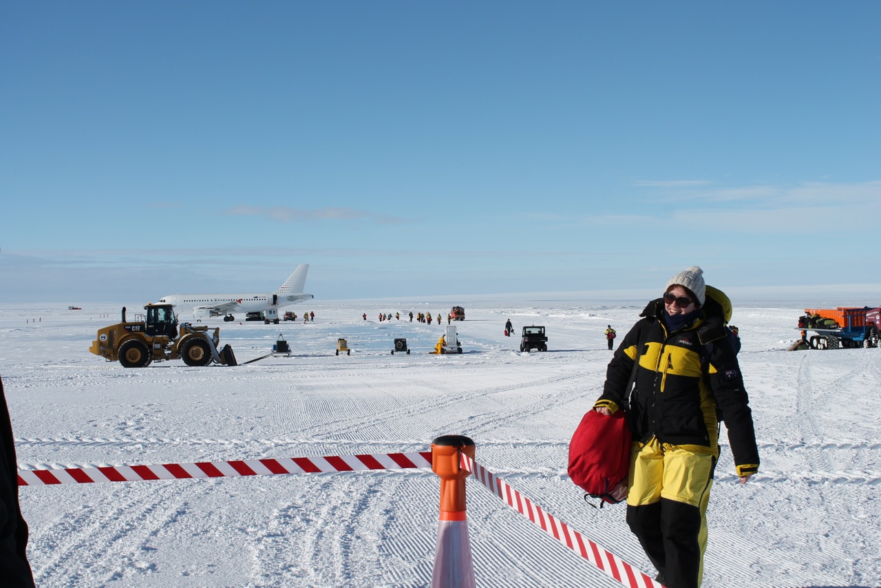
Arriving in Antarctica! The Airbus 319 is in the background, on the apron of the Wilkins blue ice aerodrome.
Antarctica is a great place to collect samples because most of the research into sea ice reconstructions are based on Antarctic ice cores and the sea ice variability is somewhat simpler than in the Arctic. I was able to go to East Antarctica to collect snow samples from the Antarctic coast in order to study how all three sea ice proxies (Sodium, MSA and halogens) respond to recently observed sea ice changes.
Getting to Antarctica is pretty easy nowadays: rather than taking a 3 week voyage on an icebreaker through the Southern Ocean, we can just fly there in 4 hours on an Airbus 319 which is chartered by the AAD. This service makes it possible to go to Antarctica, wait for a window of good weather at the sampling site, and then fly back to Australia in less than three weeks!
Driving up to Law Dome in the AAD Hägglunds tractors. The surface was smooth fresh snow which allowed us to travel up to Law Dome without too many bumps.
Setting up camp at Law Dome. The two “Häggs” are in the background. Note the perfect drilling conditions: clear skies and no wind!
Together with Tessa Vance (AAD researcher) and an expert support team we drove up to Law Dome for the sampling. Law Dome is a special zone of high snow accumulation as it receives over a metre of snow every year, and has been a site for studying sea ice reconstructions for more than 20 years. We spent two days at Law Dome, during which we drilled an 8 metre snow core and sampled surface snow around the drill site. The support team also set up a weather station, so we know more about the local conditions at Law Dome over the coming years.
Tessa drags equipment to the sampling site. We did the sampling 175 metres upwind from the camp to ensure that diesel emissions from the tractors did not disturb the samples we collected.
Logging the snow core length and storing it in plastic bags for transport back to Australia. In the background, Tessa is drilling the next sample.
The automatic weather station is now up and running. There is so much snow accumulation at Law Dome that the 7 metre high pole will need to be replaced in 3 or 4 years otherwise it will be completely buried!
The next step is to do the measurements. All three sea ice proxies (Sodium, MSA and halogens) will be measured in parallel in the snow core and snow surface samples to produce a consistent story about sea ice at the Law Dome coast over the past 5 years. These measurements will be done in Australia, in Italy and at the Centre for Ice and Climate in Denmark.
Ice2Ice members from the Bjerknes Centre recently published an article in the Journal of Geophysical Research Oceans titled “Consequences of future increased Arctic runoff on Arctic Ocean stratification, circulation, and sea ice cover.” Here you can read the corresponding author Aleksi Nummelin’s explanation of the key findings in this new article.
Scenarios with freshwater leading to sluggish currents and less heat being transported to northern high latitudes have been seen as a potential cause for rapid climate changes. In two recent studies we show that while this scenario is plausible in the North Atlantic, the ocean response in the Arctic is quite the opposite.
The scientific narrative of larger freshwater input and weaker ocean circulation is based on the extensive literature on the effects of freshwater on the ocean circulation in the North Atlantic. However, the response in the Arctic has received much less attention and this is what we were after. For simplicity we focused on changes in the river runoff, which is projected to increase as much as 30% by the end of the 21st century.
In our first study (Nummelin et al., 2015a) we used a simple column model and represented the whole Arctic as one vertical profile. In this model we increased the river runoff and found that the heat flux from ocean to the sea ice stays close to constant even though the surface layer freshens, reducing vertical mixing towards the surface from warm Atlantic origin waters at depth. This somewhat counterintuitive result follows from the reduced surface heat flux outside the ice covered areas, which leads to warmer Atlantic Water layer and a modest change in vertical heat flux inside the Arctic.
In our second study (Nummelin et al., 2015b), instead of working with the idealized column model, we wanted to try out something a bit more realistic and we turned into the Norwegian Earth System Model (NorESM1-M). We chose to force the model with a constant atmospheric state and allowed the ocean and sea ice cover to adjust to increasing Arctic runoff. This more complex model confirmed our previous result and showed that the increase in the runoff leads to warmer Arctic Ocean with very little change in the vertical ocean heat flux under the ice cover. As a result the ocean circulation turned out to be more important for the increase in the sea ice thickness than the changing vertical ocean stratification.
These two studies lead us to conclude (summarized in Figure 1) that while the North Atlantic ocean responds to increasing freshwater input with a slowdown of circulation, reduced heat transport, and a cooling of the ocean, the reduced surface fluxes (i.e. less cooling) further north accommodate the reduction in the ocean heat transport. By the time the Atlantic inflow enters the Arctic the stronger stratification and reduced mixing have lead to slight expansion of the ice cover and much warmer Atlantic water at depth. In fact the ice cover adjust preferably by increase in the ice extent, not by increase in the thickness because the vertical heat flux in the already ice covered areas stays constant due to the warmer ocean at depth.
Figure 1: Schematic of the ocean heat budget. The dashed lines show the current situation while the solid lines indicate the situation when the runoff increases. The ocean transports heat towards north and gradually loses some of its heat to the atmosphere as it goes. When the runoff increases the Subpolar Gyre cools due to reduced ocean heat transport. Further north in the Nordic Seas the ocean heat transport is still smaller, but now the surface heat flux is reduced as well, and the ocean loses less heat. Finally, in the Arctic the sea ice expands as the stronger stratification mixes less heat towards the surface, but further inside the basin the warm ocean compensates for the strong stratification keeping the surface heat flux constant. Figure: Aleksi Nummelin.
In our upcoming study we finally apply all the information we have gained from the two previous studies to understand the changes in the Arctic Ocean in the fully coupled atmosphere-ocean simulations during the ongoing century. From the preliminary results it seems that the two most important findings are similar to the idealized studies: first, changes in the North Atlantic have relatively little to do with the changes in the Nordic Seas and the Arctic, and second, ice extent responds to changes in ocean heat transport.
References
Nummelin, A., C. Li, and L. H. Smedsrud (2015a), Response of Arctic Ocean stratification to changing river runoff in a column model, J. Geophys. Res. Oceans, 120, 2655–2675, doi:10.1002/2014JC010571.
Nummelin, A., M. Ilicak, C. Li, and L. H. Smedsrud (2015b), Consequences of future increased Arctic runoff on Arctic Ocean stratification, circulation, and sea ice cover, J. Geophys. Res. Oceans, 120, doi:10.1002/2015JC011156.
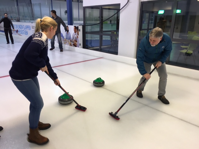
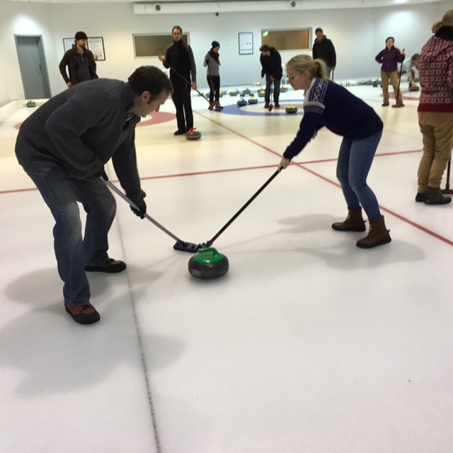
When the Bergen ice2ice team (or should I say Kerim) decided after New Year that it was about time to organise something social and fun I suggested curling. Kerim his rather simple reply (Perfect Sarah! So, you will organise it then) was all that was necessary to have a decision. Curling it was! (Lesson learned: Be careful when you suggest something)
Nonetheless, a few weeks later on a rainy tuesday evening it was time to play some curling. Fourteen of our ice2ice colleagues, including a guest from Copenhagen (Markus) took the bus to Iskanten Ishall. Of course, after a long working day we were all very hungry and needed some pizza first. One of the conversation topics during dinner was that curling seems so easy on television, it can´t be that difficult. However, once on the ice it turned out to be slightly different. An instructor explained us the basics to play, the rules and some tricks on how to curl the stones.
Afterwards we played several games where the stones most of the times went to fast or too slow. And I guess it was the latter that caused the most laughter, because seeing your teammates swipe like crazy is kind of funny.
There is a vacancy for a PhD postion at The Department of Earth Science, University of Bergen (http://www.uib.no/geo) within the field of climate dynamics/paleoclimate. The position is for a fixed-term period of 3 years. The successful candidate will be part of the Bjerknes Centre for Climate Research (http://www.bjerknes.uib.no) and the ice2ice project (Arctic Sea Ice and Greenland Ice Sheet Sensitivity) which is an ERC-synergy project with Uni Research, the University of Copenhagen and the Danish Meteorological Institute as partners.
About the project/work tasks The focus of ice2ice is to investigate the cause and future implications of past abrupt changes in Arctic sea ice and climate on the Greenland ice sheet. The candidate will work within the field of climate dynamics/paleoclimate. The research fellow will work
Ship-board core measurements for creating an initial time scale for the cores (Photo Jørund Strømsøe)
on proxy based reconstructions and chronology of oceanographic parameters adjacent to Greenland based on geochemistry and microfossils.
As part of the PhD program the candidate is expected to conduct a research stay at the ice2ice partner institution in Copenhagenor at one of the other collaborating institutions in the project.
Qualifications and personal qualities
The applicant must hold a master’s degree or the equivalent in physics, mathematics, earth science (including geology, climate, meteorology, oceanography) or similar relevant fields, or must have submitted his/her master’s thesis for assessment prior to the application deadline. It is a condition of employment that the master’s degree has been awarded.
Should have a suitable background in paleoclimatology, preferably based on sediment records
The ability to work independently as well as in interdisciplinary research groups.