Every second month the DMI and NBI groups meet to discuss progress within the ice2ice frame. During these meetings we discuss progress within individual projects, model runs needed, but also more practical issues, such as when next to meet.
Thursday March 17th we had a great meeting with a lot of science discussion. A summary of some of the presented material and project ideas can be found below with a headline for each individual presenter. Besides the four speakers below, Martin Olesen also gave an update on his work.
1420 year long climate change run at DMI
by Shuting Yang
A 1400-year long climate change simulation had been performed using the fully coupled climate model-Greenland ice sheet model system, EC-Earth – PISM model at the DMI’s previous HPC system, in order to investigate the evolution of the Greenland ice sheet in a changing climate, and its feedback to the climate system. The long simulation followed the CMIP5 historical and extended RCP8.5 protocol starting from the preindustrial condition at 1850 and spanned to 3269. We examined briefly the characteristics of the climate and the Greenland ice sheet in this long simulation. A number of research topics are suggested and further investigations have been evolved.
Signal transmission in Ocean General Circulation Models
by PhD Mads Bruun Poulsen
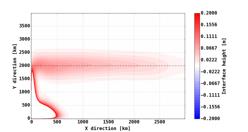
Observations suggest that there exists an anti-phase relationship between the climate of the northern and southern hemisphere during Dansgaard-Oeschger (DO) events. A complete explanation for DO events thus needs to encompass the story of why there is an inter hemispheric climate response. One way to assess the physics is through experiments using General Circulation Models (GCM), but this approach relies on that the model in use is able to resolve the waves that convey the climate signal. The ocean in particular is believed to play a role in the process of transmitting the signal through Kelvin and Rossby waves. The figure displays the model results from a simple shallow-water model in a domain that is thought to represent the equatorial region of the abyssal Atlantic Basin. It is seen how a Kelvin wave is travelling eastward along the equator, setting up the deep circulation. It is the desire to project these results from a simple model onto a more complex ocean GCM.

What is driving the mass flux variability at the NEGIS outlets.
by PhD Nicholas Rathmann
The dynamic mass loss from marine terminating outlet glaciers is a significant contribution to the current mass budget of the Greenland ice sheet. Using the Uá shallow shelf approximation model together with new ESA CCI GIS surface velocity maps, this study presents initial results on the current seasonal variations of basal properties of the marine outlets of the Northeast Greenland ice stream, one of which recently has been found to exhibit an accelerated retreat since 2012. Furthermore, the groundwork is laid out for future work on correlating such changes with climatic parameters and determining possible impacts on the up-stream catchment area.

Permafrost modeling for southwestern Greenland
by PhD Christian Rodehacke
As part of Danish Arctic activities in the Arctic, scientific observations and modeling estimates of various kind are provided to the interested public under www.PolarPortal.dk. As a new effort the Danish Meteorological Institute plans to use the in-house high resolution weather forecast model of the Greenlandic territory to drive the Permafrost model GIPL with the computed atmospheric information. The permafrost model is used in a close collaboration with the Geophysical Institute Permafrost Laboratory (LINK for the Institute name: http://permafrost.gi.alaska.edu/about) in Fairbanks, Alaska, USA.
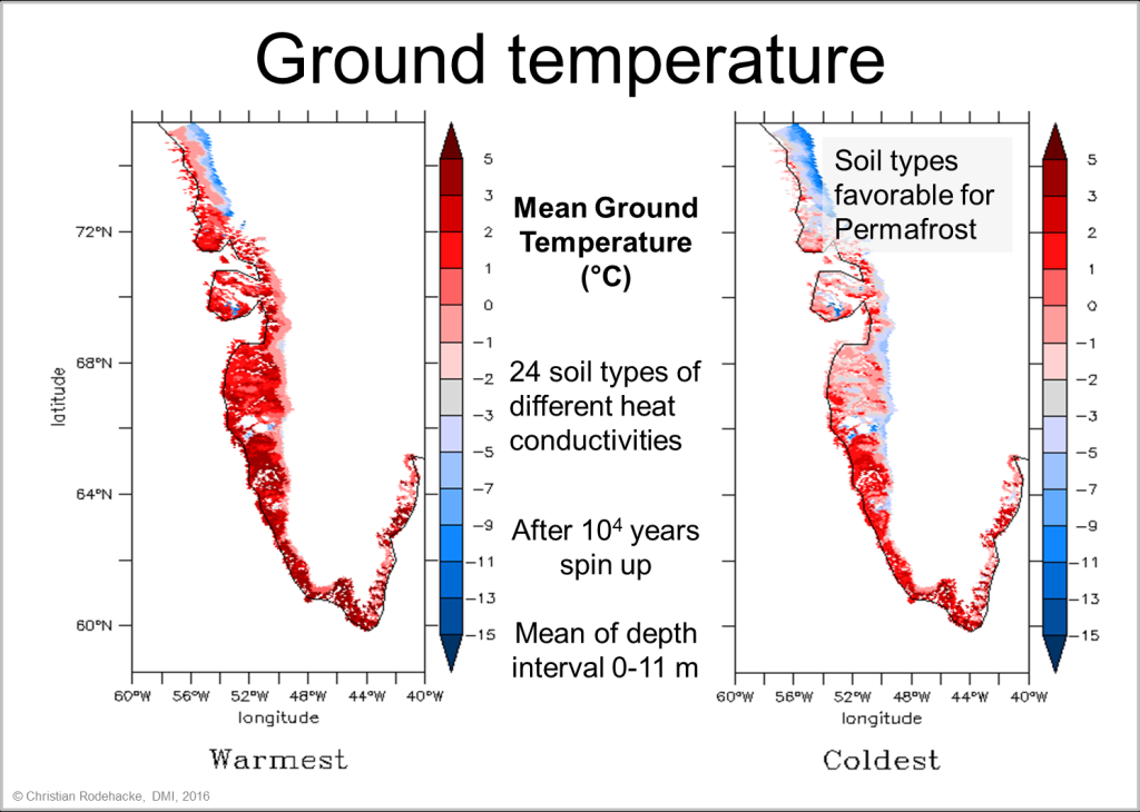
As an initial study we simulate the ground temperature in the southwest part of Greenland. At each grid location we consider 24 different soil profiles that differ in the layering of soil texture, soil material, pore space, water content, and thermal properties. These ground properties determine strongly the heat flow in the ground and, ultimately if permafrost is present. The figure shows the distribution of the computed mean ground temperature in the upper 11 meters in red-blue colors (see colorbar) while the black line follows approximately the coast. The left subfigure depicts the ground temperature where the ground properties generate maximal temperature at of each grid point; the ground properties support a warm ground. The right subfigure shows instead the corresponding minimal temperature in the ensemble of 24 soil types. In this case the layering of ground properties favor permafrost conditions. This example highlights both the need to choose adequate soil properties to simulate permafrost conditions, and, for unknown ground conditions, to compute the conditions for various types to delimit the range of expected ground temperatures.
